Protocol 1
Quick (between 6 - 7.5 minutes) protocol to locate the rough location of the receptive field and preferred contrast of the cell.
- Aim 1: Find which flash location elicits the greatest response.
- Aim 2: Determine whether the cell shows a preferred contrast to dark or light flashes.
Use this location and preferred contrast to create and run protocol 2 (P2).
Overview:
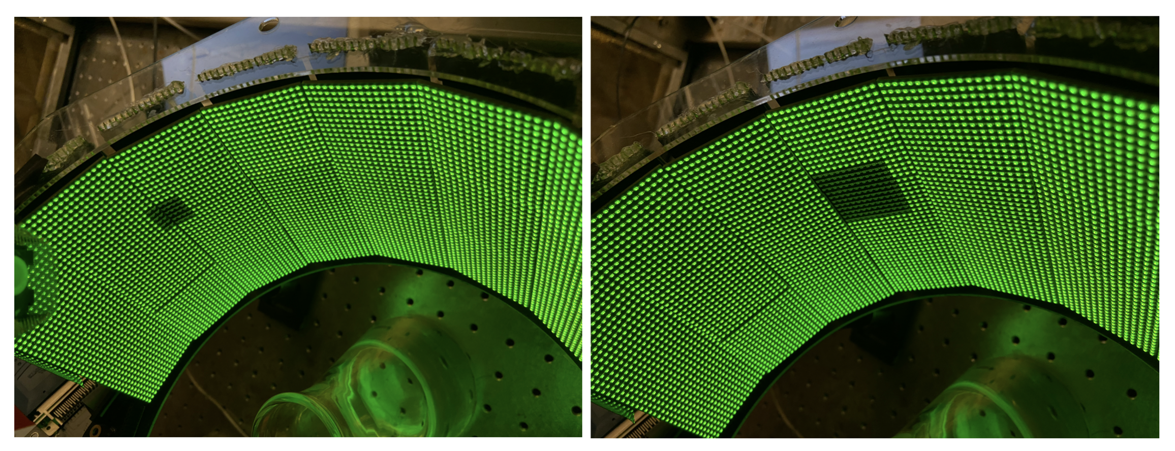
Flickering squares of two different sizes (12 x 12 pixels and 6 x 6 pixels) are presented on one half of the arena screen (either left or right half). Both dark and bright squares are presented in an alternating order. The order of presentation is designed to avoid consecutive flashes appearing close enough to each other that they would activate the same cell’s RF. These stimuli are repeated 4 times.
Location: The current most-up-to-date version of P1 can be found within the nested_RF_stimulus GitHub repository in protocols/bkg4/LHS and protocols/bkg4/RHS folders.
Intensity values: These protocols have a background pixel intensity value of 4 (out of 15), dark stimuli have a pixel value of 0 and bright stimuli have a pixel value of 15.
Stimulus parameters: Each protocol consists of both dark and bright flashing squares of 12 x 12 pixel size and then 6 x 6 pixel size that are presented on a non-overlapping grid on one half of the arena screen. One half of the arena relates to an area of 6 x 3 panels (16 x 6 = 96 pixels wide, 16 x 3 = 48 pixels high). In the G4 ephys LED panel setup each pixel is 1.25 degrees of visual anlge per pixel. So, a 12 pixel square is 15 degrees of visual angle, and a 6 pixel square is 7.5 degrees of visual angle. Each flash is presented for 200ms with an inter-flash interval of 150ms.
The schematics below show the complete flash grids as presented on the arena. Each coloured square is one flash position, and together they tile one half of the arena screen without overlap.
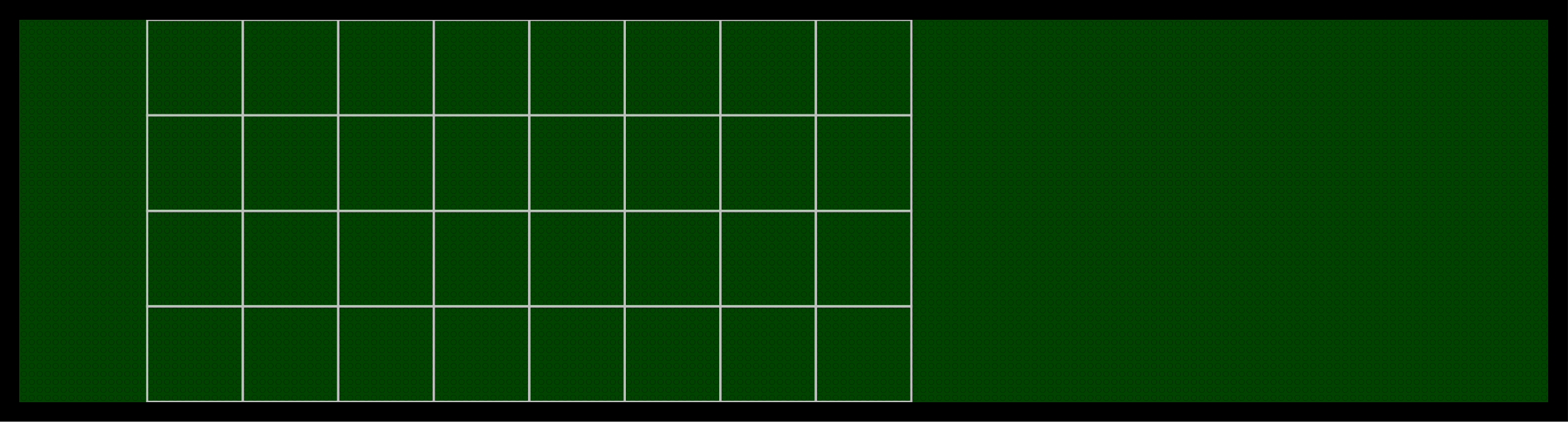
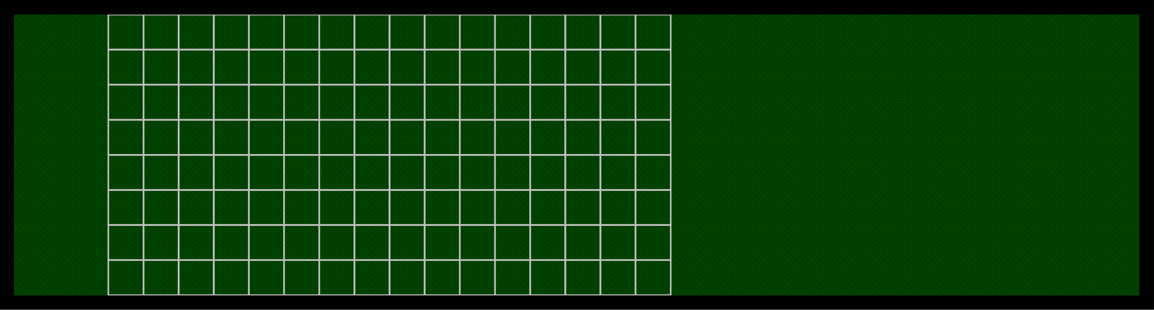
Protocol design: The protocol starts with 5s of a full field greyscale frame at the background value intensity for 5s, then runs through the larger 12 x 12 pixel flashes first, then the smaller 6 x 6 pixel flashes. The order in which the flashes are presented is not random, but was designed to avoid consecutive flashes appearing close enough to each other that they would activate the same cell’s RF. These stimuli (5s static grey + 12 pixel bright and dark flashes + 6 pixel bright and dark flashes) are repeated 4 times.
Flash presentation: The flashes are presented so that dark and light flashes are shown alternately. To try and explain how the flashes are presented: the screen was divided into 4 quadrants, then a dark flash is presented in the lower left corner of the top left quadrant, then a light flash in the lower left corner of the top right quadrant, then a dark flash in the lower left corner of the bottom left quadrant, and finally a light flash in the lower left corner of the bottom right quadrant. This is then repeated for the adjacent flash position in each quadrant, and repeats until both dark and light flashes have been presented in all positions on the screen.
Analysis plots: In order to process the data from P1, a processing_settings.mat must be generated and fed in to the G4_experiment_conductor. The function create_processing_settings.m within the G4_Data_Analysis repository can be used to create this file. In order to analyse the flash data from P1 the parameter settings.is_ephys_grid must be set to 1, along with the accompanying parameters for grid processing: neutral_frame, grid_columns and grid_rows.
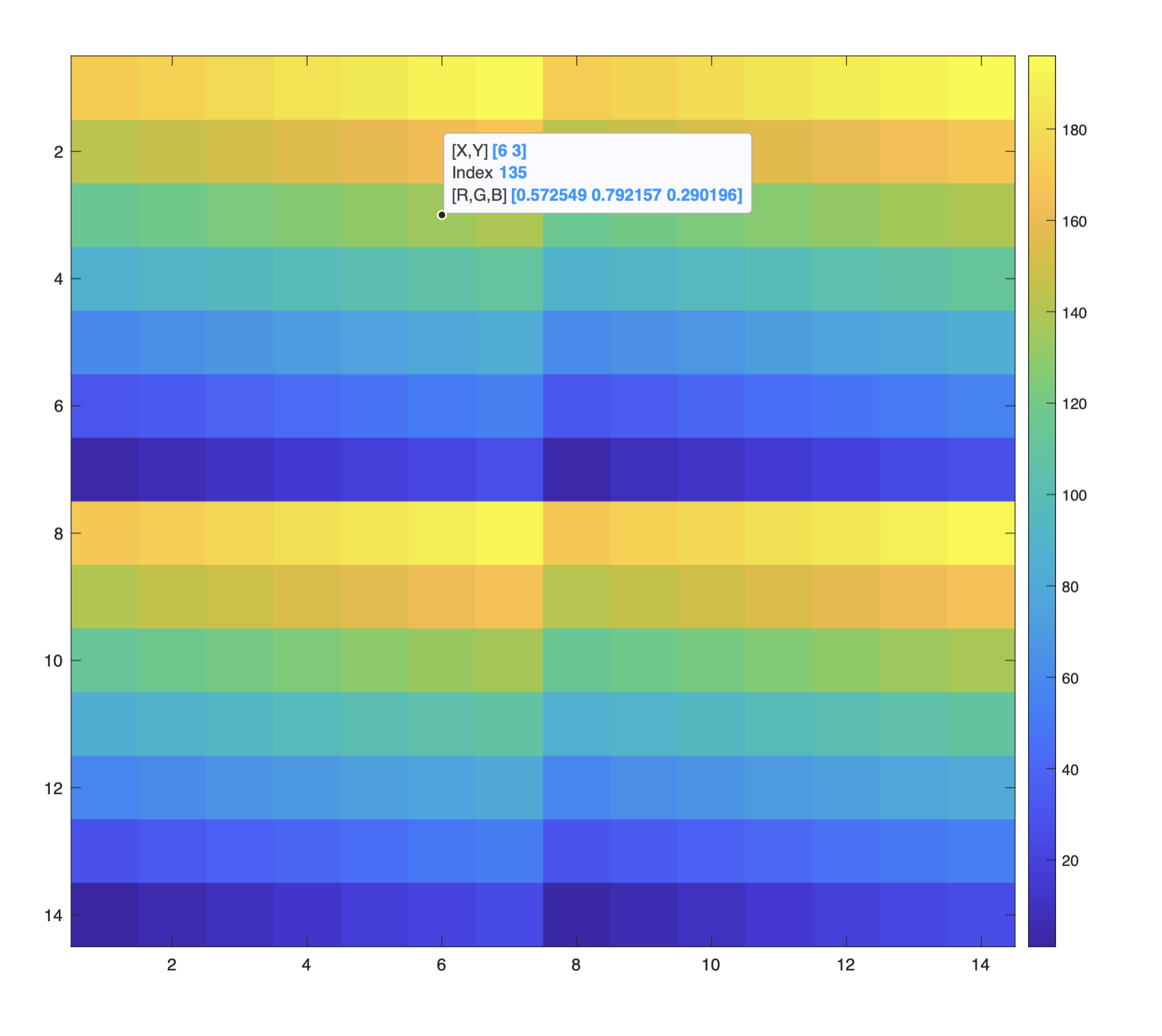
When settings.is_ephys_grid is equal to 1, then when the experiment conductor runs the function process_data, this function will then run the function ephys_grid_processing.m (link to the GitHub repo here) which will then generate the example plots shown below.
Four plots will be generated, one for each flash size and contrast combination (12 pixel bright, 12 pixel dark, 6 pixel bright, 6 pixel dark). The number above the plot with the maximum response for the 6 pixel flashes should be noted down, as this will be the peak_frame value that is input into the generate_protocol2() function to create P2.
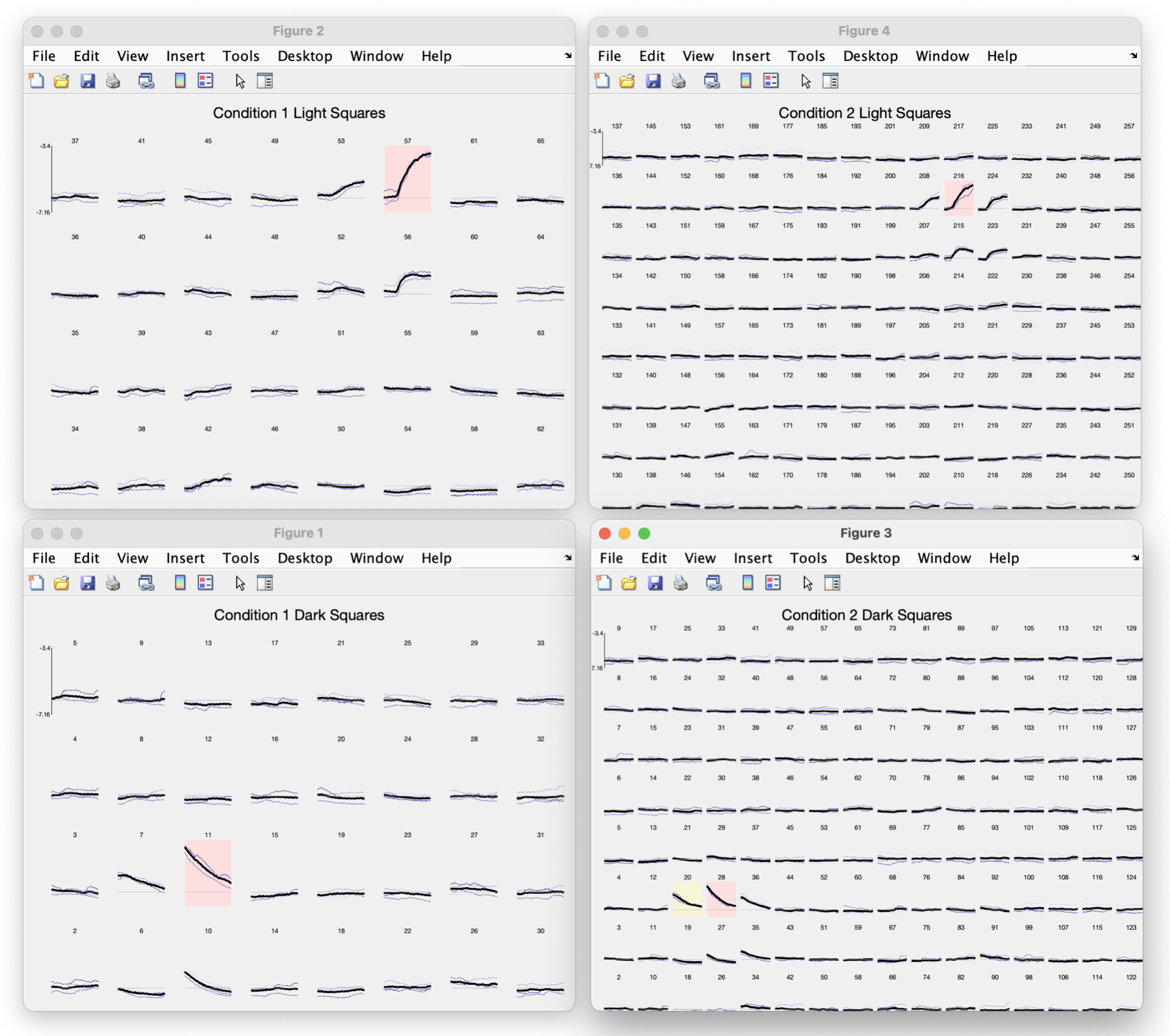
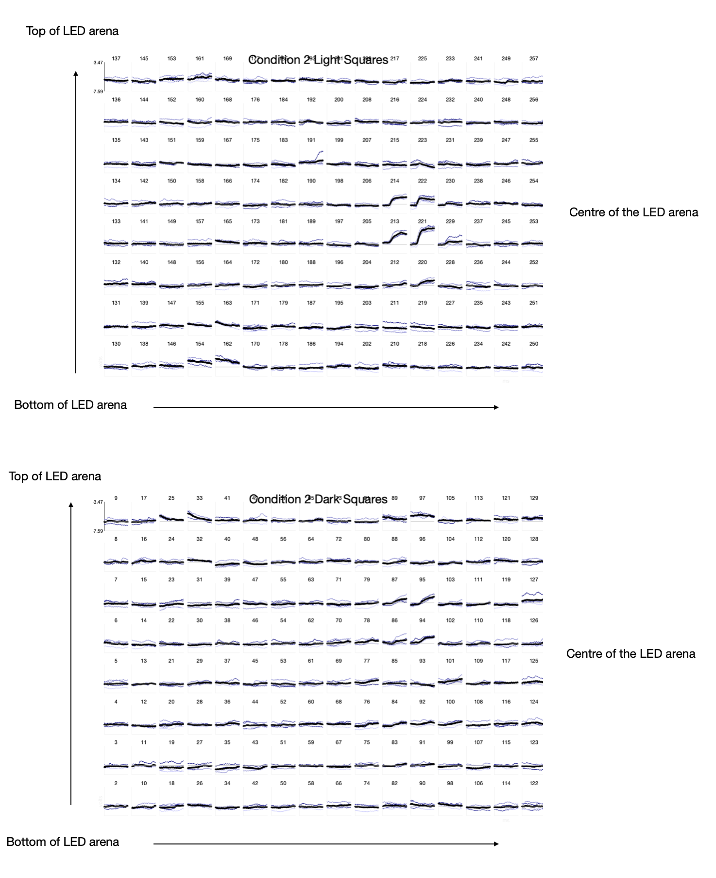
Enlarged view of example plots generated after running P1.
generate_protocol2().What to look for in the P1 results
After running P1, use the four grid plots to determine:
Which contrast elicits the largest response? Compare the bright and dark flash plots. If the cell responds more strongly to bright (ON) flashes, it is likely an ON-pathway cell (e.g. T4). If it responds more to dark (OFF) flashes, it is likely an OFF-pathway cell (e.g. T5). This determines whether you run the ON or OFF version of Protocol 2.
Where is the receptive field? Look at the 6 pixel grid plots (both contrasts) and identify which subplot has the largest response. The number above that subplot is the
peak_framevalue you will enter when runninggenerate_protocol2().Is the RF too close to the edge? If the
peak_framecorresponds to a flash position within ~15 pixels of the arena edge, the 30 x 30 pixel stimulus area used in Protocol 2 may extend beyond the arena boundary. In this case, it may not be worth running Protocol 2 — the code will display a warning if this occurs.Is the recording quality sufficient? If the responses are noisy, inconsistent across repetitions, or very small in amplitude, it may indicate a poor recording that is not worth pursuing with Protocol 2.