Flash analysis
Stimulus overview
The flash stimuli in Protocol 2 consist of small squares presented on a 50% overlapping grid within the stimulus area. Two sizes are used: 4 pixel and 6 pixel squares.


Breakdown of process_flash_p2
function process_flash_p2(exp_folder, metadata, PROJECT_ROOT, resultant_angle)This function processes the responses to the square flash stimuli in Protocol 2. It takes in resultant_angle (the preferred direction from bar sweep analysis) to overlay a direction arrow on the receptive field plots. All results are saved to disk — the function does not return any values.
Loading the data
The frame position and voltage data are loaded from the experiment Log file, as in the bar sweep analysis. The voltage is multiplied by 10 (reversing the acquisition hardware scaling) and the median voltage is computed as a baseline. A smoothed version of the voltage is also computed with movmean(v_data, 20000) for use in parsing.
The function loops through both flash sizes (4 pixel then 6 pixel), running the parsing, plotting, and metric extraction steps independently for each.
Parsing the flash data
The function parse_flash_data extracts the flash responses from the full recording. It requires on_off, slow_fast, and px_size as inputs.
Step 1 — Find the repetition boundaries.
The parser uses frame position transitions to locate the start of each flash block. The key difference between ON and OFF versions of P2 is the starting frame number:
| Stimulus | OFF version (f_data value) |
ON version (f_data value) |
|---|---|---|
| First 4px flash | 1 (frame 2 of pattern) | 197 (after 196 dark frames) |
| First 6px flash | 1 (frame 2 of pattern) | 101 (after 100 dark frames) |
The end of the 4 pixel block is identified by the start of the 6 pixel block. The end of the 6 pixel block is found using the same large frame-drop method used in bar data parsing (stored in idx_6px).
Step 2 — Find individual flash start times.
Within each repetition range, start_flash_idxs is generated by finding timepoints where the frame position difference is > 0 (each flash onset). For each flash, the data extraction window spans from 1,000 datapoints before the flash start to 6,000 datapoints after (7,000 total at 10 kHz). Since each flash lasts 160ms with a 440ms interval (600ms total = 6,000 samples), this window captures one complete flash-plus-interval cycle with a pre-stimulus baseline.
The data is stored in three arrays, all of size [n_reps, 7000]:
data_frame— frame position datadata_flash— median-subtracted voltage datadata_flash_raw— raw voltage data
Step 3 — Compute metrics per flash position.
For each flash position, the following metrics are computed from the mean response across repetitions:
max_data— 98th percentile of the voltage during the flash presentation window (from 500 samples after flash onset to the end of the extraction window for slow flashes).min_data— 2nd percentile of the voltage during the second half of the flash presentation window (from 2,500 samples after flash onset onwards). This captures delayed inhibitory responses.diff_mean— difference between max and min response:max_data - min_data.
These values are used to classify each flash position into one of three response groups:
cmap_id |
Classification | Condition |
|---|---|---|
| 1 | Excitatory | |
| 2 | Inhibitory | |
| 3 | Neutral | Response below threshold |
The data_comb array stores the representative value for each flash position:
cmap_id = 1→ max voltage (excitatory peak)cmap_id = 2→ min voltage (inhibitory trough)cmap_id = 3→ mean voltage across the last 25% of the flash period
Two variance metrics are also returned:
var_across_reps— coefficient of variation (CV) across the 3 repetitions, measuring response reliability.var_within_reps— CV within each repetition, measuring how different the response is from baseline.
The flash frame numbers are mapped to grid positions using:
rows = n_rows_cols - mod(flash_frame_num - offset, n_rows_cols)
cols = floor((flash_frame_num - offset) / n_rows_cols) + 1
All outputs are returned as square arrays of size [n_rows, n_cols] (14×14 for 4px flashes, 10×10 for 6px flashes).
Plotting the flash data
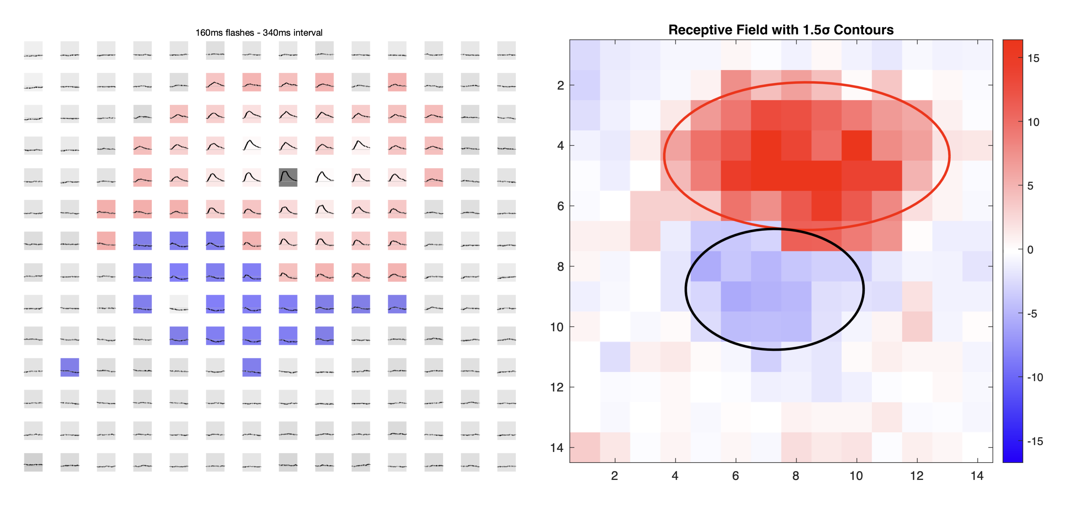
1. Grid timeseries plot — plot_rf_estimate_timeseries_line
This figure shows the mean voltage timeseries for each flash position, arranged spatially to match its screen location. The subplot background colour indicates the response classification:
- Red (cmap_id = 1) — excitatory response. Darker red = stronger depolarisation.
- Blue (cmap_id = 2) — inhibitory response. Darker blue = stronger hyperpolarisation.
- White/grey (cmap_id = 3) — no significant response.
Background intensity is proportional to the normalised data_comb value (0–1). The resultant_angle from bar sweep analysis is overlaid as an arrow indicating the cell’s preferred direction.
2. Heatmap plot — plot_heatmap_flash_responses
Creates a 2D heatmap of the normalised data_comb values using a red-blue colourmap. The colourmap is centred around the median value so that the median appears white, giving a balanced colour range:
med_val = median(data_comb(:));
clim([med_val-0.5 med_val+0.5])
Gaussian receptive field fitting
The function gaussian_RF_estimate fits a rotated 2D Gaussian to the spatial response pattern, separately for the excitatory and inhibitory lobes. It uses the built-in MATLAB function lsqcurvefit for optimisation.
Preprocessing: The data is log-transformed before fitting to reduce the influence of outlier positions: zData = sign(z) * log(1 + |z|).
Model: The fitted Gaussian has 7 parameters:
\[G(x,y) = A \cdot \exp\left(-\frac{[(x-x_0)\cos\theta + (y-y_0)\sin\theta]^2}{2\sigma_x^2} - \frac{[-(x-x_0)\sin\theta + (y-y_0)\cos\theta]^2}{2\sigma_y^2}\right) + B\]
| Parameter | Symbol | Description |
|---|---|---|
opt[1] |
A | Amplitude of the Gaussian peak |
opt[2] |
x₀ | Centre x-coordinate |
opt[3] |
y₀ | Centre y-coordinate |
opt[4] |
σ_x | Extent along the primary axis |
opt[5] |
σ_y | Extent along the secondary axis |
opt[6] |
θ | Rotation angle (radians, -π to π) |
opt[7] |
B | Baseline offset |
The parameters are bounded during fitting: amplitudes ≥ 0, centres within the grid range, sigmas ≥ 0, and rotation angle between -π and π.
For the inhibitory lobe, the data is inverted (-min_data) before fitting, so the same fitting procedure can be applied to find the inhibitory Gaussian.
Outputs:
optEx— 7-parameter vector for the excitatory Gaussian fitoptInh— 7-parameter vector for the inhibitory Gaussian fitR_squared— goodness of fit for excitatory lobe:R² = 1 - (SS_res / SS_tot)R_squaredi— goodness of fit for inhibitory lobe (same formula)f1,f2— figure handles for the fitted surface plots
Saved outputs
Results are stored in a nested structure rf_results and saved as rf_results_<date>_<time>_<strain>_<on_off>.mat in the results/flash_results/ folder. The structure contains, for each flash size (rf_results.slow):
| Field | Description |
|---|---|
data_comb |
Representative response value per position (max, min, or mean) |
max_data |
98th percentile peak per position |
min_data |
2nd percentile trough per position |
cmap_id |
Classification per position (1 = excitatory, 2 = inhibitory, 3 = neutral) |
var_within_reps |
Coefficient of variation within repetitions |
var_across_reps |
Coefficient of variation across repetitions |
R_squared |
R² for excitatory Gaussian fit |
sigma_x_exc |
Excitatory extent along primary axis |
sigma_y_exc |
Excitatory extent along secondary axis |
optExc |
Full excitatory Gaussian parameters [7×1] |
R_squaredi |
R² for inhibitory Gaussian fit |
sigma_x_inh |
Inhibitory extent along primary axis |
sigma_y_inh |
Inhibitory extent along secondary axis |
optInh |
Full inhibitory Gaussian parameters [7×1] |