Bar flash analysis
Stimulus overview
Key points:
- 88 flashes in total (8 orientations, 11 flashes per orientation.)
- 88 flashes repeated 3 times in a different random order per repetition.
- Flashes are only in one contrast, either bright or dark.
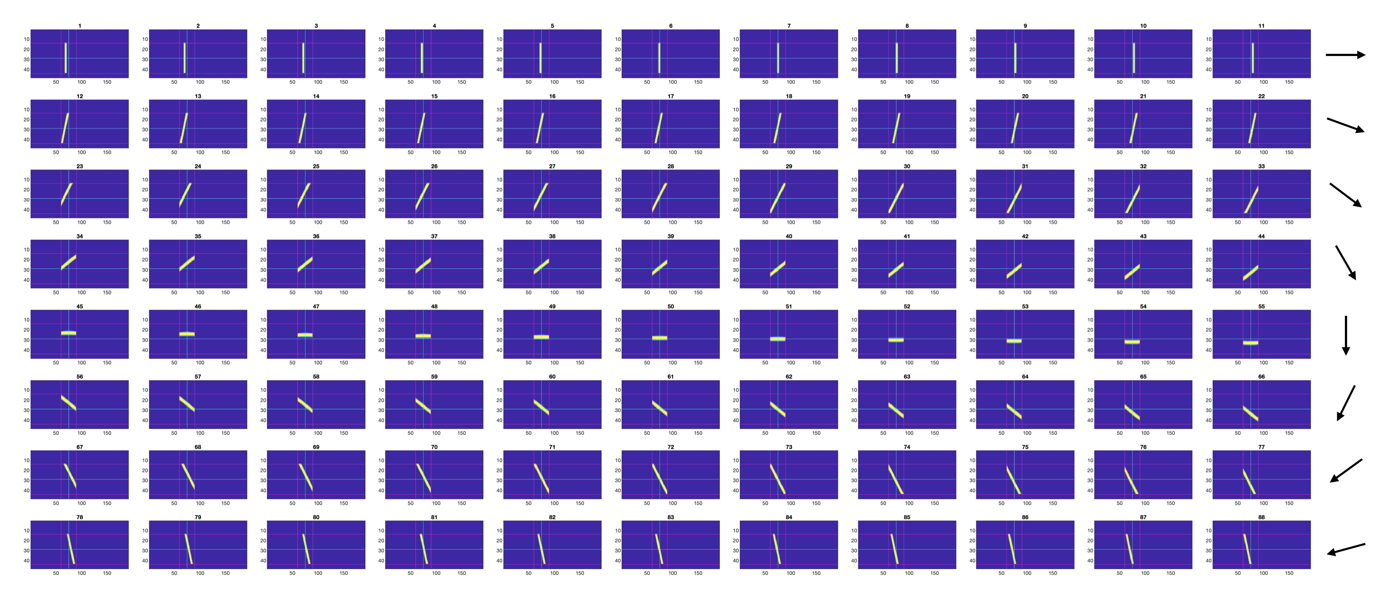
- 1 flash centred within the 30 x 30 pixel square and then 5 positions above and below that position along the axis.
- Slow flashes = 1s total each — 80ms flash with 920ms interval.
- Fast flashes = 0.5s total each — 14ms flash with 486ms interval.
Stimulus description
| Parameter | Value |
|---|---|
| Num orientations | 8 |
| Flashes per orientation | 11 |
| Step size (px) | 1 / 2 |
| Duration slow | 80ms |
| Inter-flash interval slow | 920ms |
| Duration fast | 14ms |
| Inter-flash interval fast | 486ms |
Scripts used to make the stimulus:
generate_bar_flash_stimulus_xy.m — makes the pattern.
generate_bar_flash_pos_fns.m — creates the position functions. This function makes a different position function for each repetition so that the bar flashes are presented in a random order each time.
The stimulus is made from the pre-made bar patterns within the folder C:\matlabroot\G4_Protocols\nested_RF_stimulus\results\patterns\protocol2\full_field_bars4 that are used for generating the bar sweep stimuli too. So, the pixel intensity values will match those stimuli.
Bar flash stimulus changed from 1 to 2 pixel steps per frame on October 23rd 2025.
Breakdown of process_bar_flashes_p2
function process_bar_flashes_p2(exp_folder, metadata, PROJECT_ROOT)This function processes the responses to bar flash stimuli. Unlike the bar sweep and flash analyses, no direction selectivity or receptive field metrics are computed — the primary output is the raw timeseries data and visualisation figures. All results are saved to disk.
Loading the data
The frame position and voltage data are loaded from the experiment Log file:
f_data = Log.ADC.Volts(1, :); % frame data
v_data = Log.ADC.Volts(2, :)*10; % voltage data
Parsing the bar flash data
The function parse_bar_flash_data extracts bar flash responses from the full recording.
Step 1 — Find repetition boundaries.
The parser detects 3-second gaps (≥ 30,000 samples at 10 kHz) in the frame data to identify the boundaries between stimulus blocks. These gaps correspond to the 3s grey backgrounds inserted between stimulus types within each repetition.
Step 2 — Separate slow and fast flash blocks.
Within each repetition, the slow bar flashes (80ms/920ms) are presented first, followed by the fast bar flashes (14ms/486ms), with a 3s grey gap between them. The parser uses the gap indices to locate the correct data ranges for each speed condition within each of the 3 repetitions.
Step 3 — Extract individual flash timeseries.
Within each speed block, individual flash onsets are identified by frame position transitions. For each flash, the extracted data window includes a proportion of the inter-flash interval before and after the flash itself (controlled by the parameter prop_int_2_show, default 0.75). This provides context to see the baseline voltage around each flash.
Step 4 — Organise into cell arrays.
The extracted timeseries are organised into cell arrays indexed by position, orientation, and repetition:
| Output | Size | Description |
|---|---|---|
data_slow |
11 × 8 × 3 | Slow flash timeseries (positions × orientations × reps) |
data_fast |
11 × 8 × 3 | Fast flash timeseries |
mean_slow |
11 × 8 | Mean across 3 reps (NaN-padded if lengths differ) |
mean_fast |
11 × 8 | Mean across 3 reps |
Plotting the bar flash data
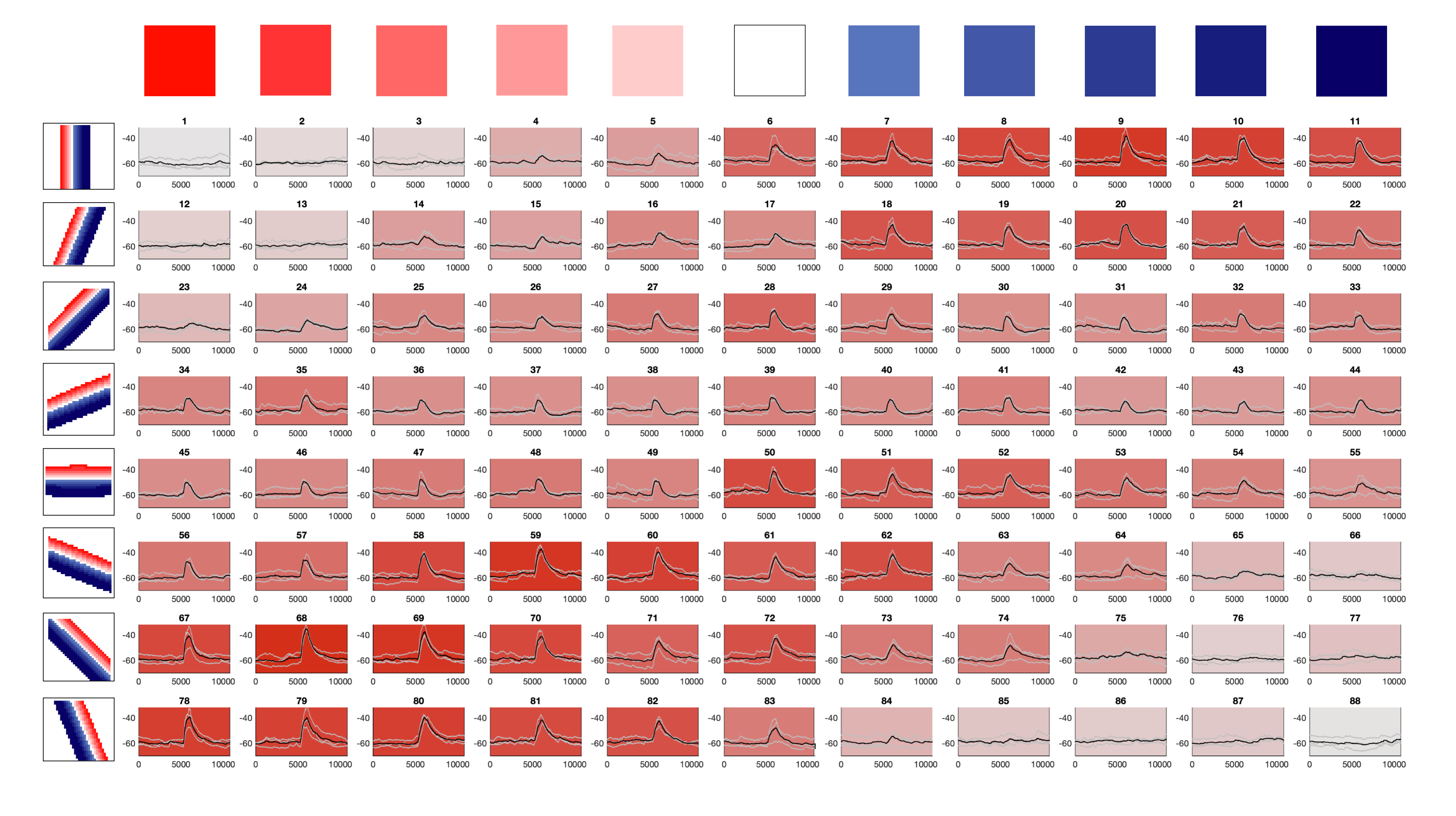
The function plot_bar_flash_data creates an 8 × 11 tiled figure (8 rows for orientations, 11 columns for positions) showing the response timeseries at every bar flash condition.
PD alignment — shiftMaxColumnTo5
Before plotting, the data is circularly shifted so that the orientation with the strongest response is centred at column 5. This function:
- Computes the peak response for each orientation (using the 98th percentile in the 40%–80% window of each timeseries).
- Identifies which orientation column has the strongest overall response.
- Circularly shifts all 8 orientation rows so that the peak column is at position 5, labelled “PD” (preferred direction).
- The opposite row (position 1) is labelled “OD” (orthogonal direction).
Subplot appearance:
- Individual repetitions are plotted in grey.
- Mean response is plotted in black.
- Vertical black lines mark flash onset and offset within each subplot.
- Background colour indicates response strength: stronger responses produce a darker red-tinted background. The colour is normalised relative to the strongest response across the whole figure using the formula
[1, norm_value, norm_value] × 0.9. - Y-axis limits are fixed at [-75, -30] mV.
Two figures are generated: one for slow flashes and one for fast flashes.
Saved outputs
Results are saved as bar_flash_results_<date>_<time>_<strain>_<on_off>.mat in the results/bar_flash_results/ folder. The saved variables are:
| Variable | Description |
|---|---|
data_slow |
11 × 8 × 3 cell array of slow flash timeseries |
data_fast |
11 × 8 × 3 cell array of fast flash timeseries |
mean_slow |
11 × 8 cell array of mean slow responses |
mean_fast |
11 × 8 cell array of mean fast responses |
Figures are saved as PDFs:
figures/bar_flash_stimuli/Bar_flashes_80ms_<date>_<time>_<strain>.pdf(slow)figures/bar_flash_stimuli/Bar_flashes_14ms_<date>_<time>_<strain>.pdf(fast)
Example output