How to analyse the data from the nested RF protocol.

Protocol 1
Protocol 2
1. How the data is organised
2. How to process P2 data
  1. Breakdown of process_bars_p2
  2. Breakdown of process_flash_p2

Protocol 1

Processing settings file…
Which boxes need to be ticked in the conductor?

After protocol 1 has finished running - the processing functions should run automatically. This runs code wihtin G4_Display_Tools - it returns LOG with data inside and it generates 4 plots (grid_ephys).

From these plots you can see the response of the cell to each flash location on the screen - both 12px and 6px and ON and OFF flashes. This protocol is mainly for the experimenter to determine where the RF of the cell is located in order to present the second protocol in the correct position. From these plots it is also possible to determine if the RF of the cell is too close to the edge of the screen, in which case it is not worth running protocol 2. You can also see if the quality of the recording is not good enough to run protocol 2.

Protocol 2

How the data is organised

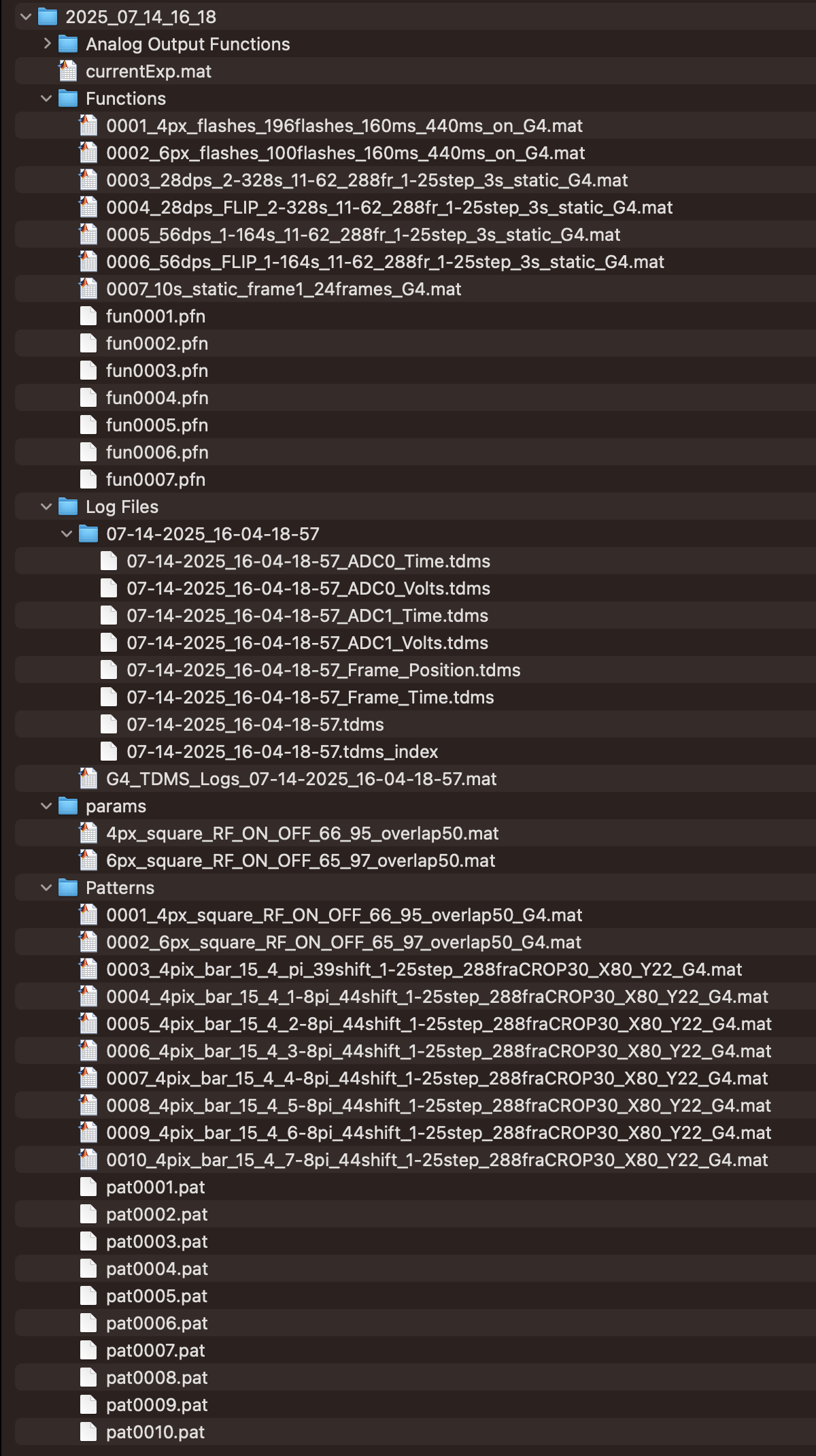
Each run of generate_protocol2() with create a new folder within C:\matlabroot\G4_Protocols\nested_RF_protocol2 with the format “YYYY_MM_DD_HH_MM” of the date and time when the protocol was run.
Within this folder there will be a patterns folder with the patterns that were used in the protocol, a functions folder with the position functions that were used, and a params folder containing a file with metadata about the protocol run.
There will also be a folder Log Files, this itself will contain a subfolder with the exact date and time of the run that will contain the raw tdms files of the electrophysiology data and the frame position data. Witin generate_protocol2() there is a function run_protocol2() that runs the protocol created. At the very end of this function there is a function called G4_TDMS_folder2struct(log_folder) - another function from the G4_Display_Tools that will convert the tdms files into a combined structure (called Log) that can be used for analysis.

Folder and file organisation for one P2 experiment.

How to process P2 data

Run the function src/analysis/process_protocol2() within the experiment folder (data/YYYY_MM_DD_HH_MM). This function reads in the metadata file that has information about the strain of the fly, peak_frame, side of the arena.

The responses to the moving bar stimuli are processed first, since this analysis generates a vector sum of the responses of the cell to bars moving in the 16 different directions. The resultant angle of this vector sum is then fed in to the function that processes the flash responses and overlays an arrow with this direction on top of the receptive field plots.

Breakdown of `process_bars_p2`

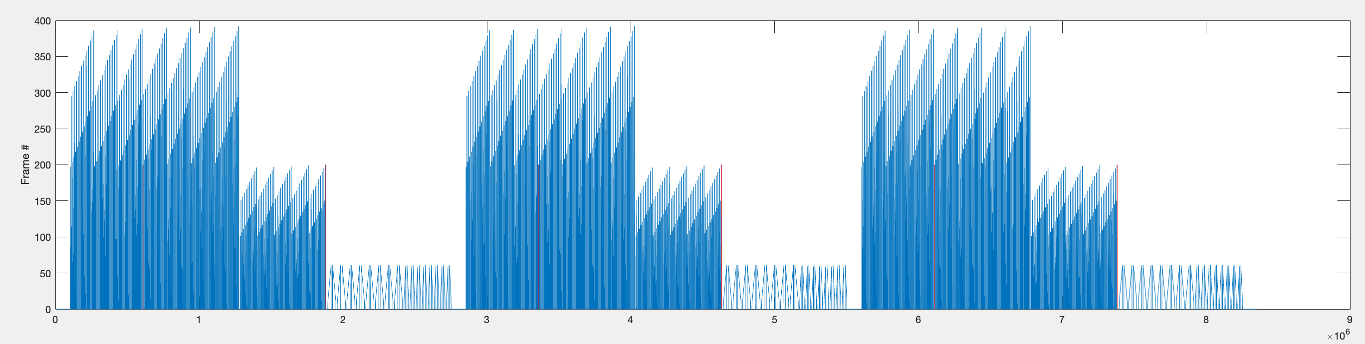
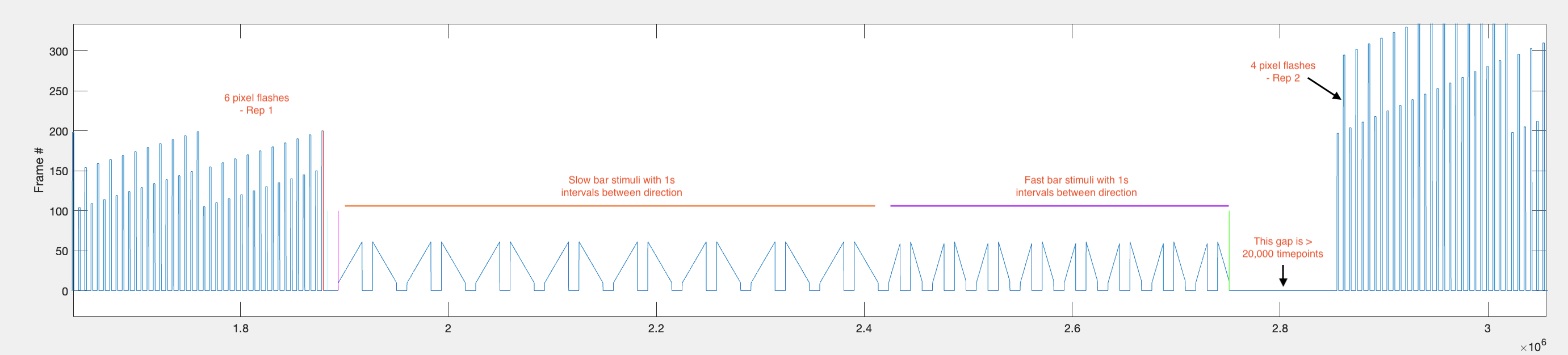
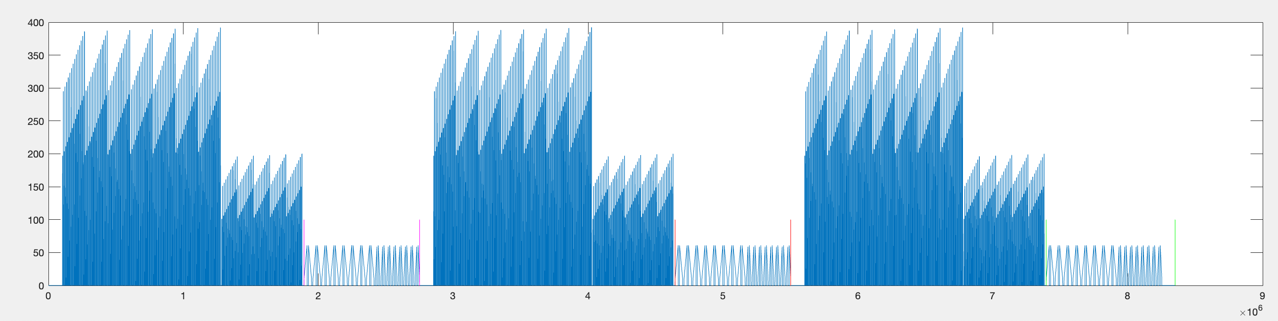
This function reads in the frame data: f_data = Log.ADC.Volts(1, :); % frame data and then the voltage data: v_data = Log.ADC.Volts(2, :)*10; % voltage data

This is the data across the entire experiment, the three repetitions of the two flash stimuli and the two bar stimuli. The voltage data is multiplied by 10 because during the data acquisition it is downsampled by a factor of 10. (TODO: ADD WHY).

[ PNG - 0001 ] ^General plot of f_data and v_data

Parsing the bar data

The function src/analysis/protocol2/pipeline/parse_bar_data is used to parse the frame data to understand when the moving bar stimuli were presented.

Find the range of timepoints during which all of the bar stimuli for each repetition were being presented. This includes both the slow and fast bars.

Firstly, using the value of the parameter on_off, which refers to whether bright (‘on’) or dark (off’) stimuli were used during the protocol, the parameter drop_at_end is set to either ‘-200’ for on_off == ‘on’ or ‘-100’ for on_off == ‘off’.

Then idx is set to the timepoints for which the difference in the frame position is equal to drop_at_end. This happens both once during the 4 pixel flashes and for the last timepoint of the last 6 pixel flash. The 1st, 3rd and 5th values are removed to remove the timepoints during the 4 pixel flashes and so only the timepoints corresponding to the end of the 6 pixel flashes remain. This is useful because this is the stimulus before the bar stimuli start.

idx = find(diff_f_data == drop_at_end);
idx([1,3,5]) = [];

MATLAB figure of the frame position data over the entire P2 experiment (blue) with vertical lines indicating the 6 timepoints in the variable 'idx' (red).

Since each flash stimulus is followed by a 440ms gap, and each bar stimulus is preceded by a 1000ms gap, there is a ~1440ms period before the first bar stimulus being presented and the last of the 6 pixel flashes being shown.

Zoomed in view of the figure above showing only the second timepoint in 'idx' that corresponds to the end of the last 6 pixel flash in Rep 1.

Ultimately, the data will be broken up into chunks of the same length with 1000ms before the bar stimulus and until 900ms after the end of the bar stimulus, but first we want to find the range of timepoints during which ALL bar stimuli (both slow and fast) are presented for each repetition.

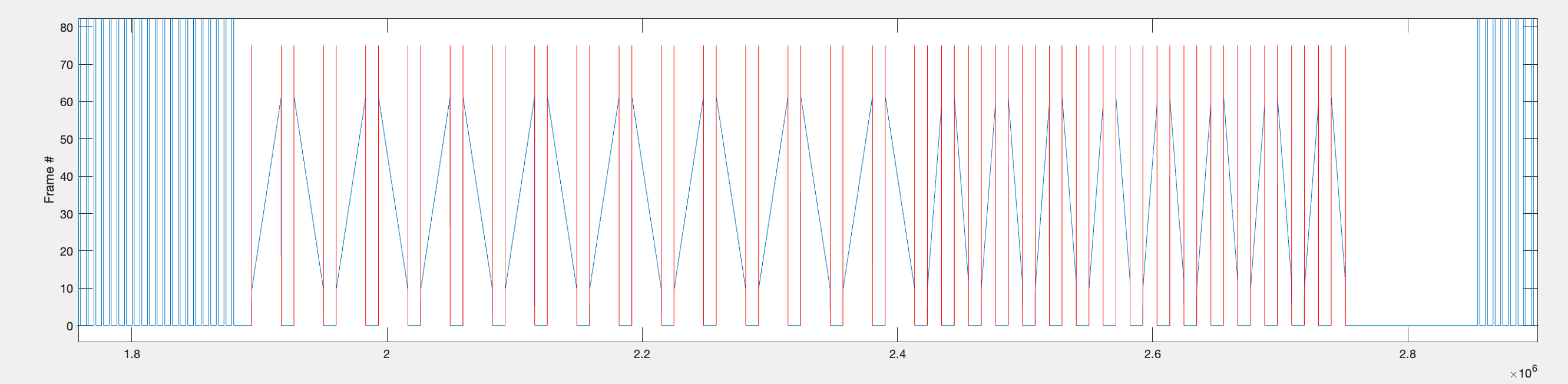
Zoomed in view of frame position data. (Red) Last frame of the last flash of the 6 pixel flashes from Rep 1. (Cyan) Time point after 440ms gap after the last flash and 1000ms before bar stimulus starts. (Magenta) First frame of the first bar stimulus in Rep 1.

The vertical bars are the timepoints that are found in the code. The two timepoints that represent the start and end of the first repetition of bar stimuli are defined as rep1_rng and are represented graphically by the magenta vertical bar and the green vertical bar. This range excludes the interval periods before the stimuli start and after the stimuli stop.

Overview of how the timing of the moving bar stimuli are found using the frame position data. The figure shows the end of the 6 pixel flashes, both bar stimuli and the start of the second repetition of the 4 pixel size flashes.

This is the code that was used to plot the cyan, magenta and green lines: plot([idx(1)+gap_between_flash_and_bars idx(1)+gap_between_flash_and_bars], [0 100], 'c') - 1000ms before the start of the first moving bar stimulus.
plot([start_f1 start_f1], [0 100], 'm') - first frame of the first moving bar stimulus.
plot([end_f1 end_f1], [0 100], 'g') - last frame of the last moving bar stimulus of the repetition.

Range of timepoints for the bar stimuli in rep1 (magenta lines), rep2 (red lines) and rep3 (green lines). The third rep uses the last frame of the experiment as the end of it's range. It doesn't matter that this includes the interval time at the end because the actual start and stop times of the bar stimuli are found within these ranges in the next step.

Find the timepoints for when each individual bar stimulus starts and stops.

Now that we have extracted the range of timepoints during which all of the bar stimuli of one repetition are presented, we now want to extract the timepoints for each individual bar stimulus (one sweep of the bar) within each repetition. To do this, the difference between frame positions are used again. This time we are looking for the timepoints when the frame position changes from 0 (the background interval frame) and a frame when the bar is being presented. For all moving bar stimuli, the bar first appears around frame 10, therefore an absolute difference of >9 in frame position was used to find the timepoints when the bar starts and stops.

Frame position over one repetition of all of the moving bar stimuli. Red vertical lines indicate the start and end of each individual flash sweep. These values are stored within 'idxs_all{1,1}'

Create the cell array data which combines the voltage data for each bar stimulus including 9000ms before and after each sweep of the bar.

The indices found above and stored in idxs_all are then used to extract the relevant voltage data for each bar sweep. Since there is a 1000ms gap between each bar sweep (added in July 2025), 900ms is added before and after the bar sweep timepoints to see the baseline voltage between each sweep.

[ PNG - 0008] ^ Frame position (blue) and the magenta vertical lines show the range of data that is included for the first bar and the cyan vertical lines show the range of data to include for the second bar. These ranges include 900ms before and after the bar stimulus itself.

This data is combined into the [32 x 4] cell array data. The voltage data for the slow bar stimuli are in rows 1:16 and the voltage data for the fast bar stimuli are in rows 17:32. Each cell contains a linear array of the voltage over the 900ms before the bar stimulus, the bar stimulus presentation and 900ms after the bar stimulus. This means that the slow bar stimuli have voltage data arrays of roughly [1 x 41100] timepoints (10kHz acquisition - 0.9s pre, 2.3s stim, 0.9s post = ~4.1s total) and the fast stimuli of [1 x 29100] timepoints (10kHz acquisition - 0.9s pre, 1.1s stim, 0.9s post = ~2.9s total). The first three columns contain the data for each repetition to each condition adn the fourth column is the mean across the three repetitions. The size of the linear arrays are trimmed to the length of the shortest repetition, concatenated and then averaged using mean().

[ PNG - 0009] ^ Example data cell array.

The cell array data is returned by the function parse_bar_data and is used for plotting and analysing the responses to the bar stimuli.

Plotting the bar data

Circular timeseries plot with central polar plot for both speeds. (src/analysis/plotting/plot_timeseries_polar_bars)

This function plots the timeseries voltage data per condition for each repetition in light grey and the mean response across conditions in light blue for the fast stimuli and dark blue for the slow stimuli. These timeseries plots are positioned in a circle, with each plots position corresponding to the direction in which the bar stimulus was moving. For instance, the plot at the very top of the circle (N position on a compass) corresponds to the response of the cell to a horizontal bar moving from bottom to top. Whereas, the plot at the right of the circle (E position on a compass) corresponds to the response of the cell to a vertical bar moving from left to right. These timeseries plots include the 900ms of interval beforehand and 900ms after the end of the bar stimulus. Thin vertical black lines are added onto the subplot to show these times.

A polar plot is positioned in the centre of the timeseries plots. To generate the polar plot, the maximum of the mean response of the cell to each direction is calculated, the median voltage across the entire recording is subtracted from this value, then it is used as the magnitude of the polar plot. Specifically, the mean response across all repetitions for each condition is extracted. This data is then trimmed to exclde the 0.9s interval before and the last 0.7s of the interval after the flash. Then, the 98th percentile value from this trimmed data is found. This value is added to the array max_v which is the size [n_conditions, n_speeds] - so in this case [16 2]. The minimum value (2nd percentile value) in the second half of this trimmed data is stored in a similar way into the array min_v. These arrays are returned by the plotting function.

[ PNG - 0010] ^ Circular timeseries + polar plot. Two colours = different speeds.

Polar plot with vector sum resultant angle arrow (src/analysis/plotting/plot_polar_with_arrow)

Plots the same polar plot as the one in the centre of plot_timeseries_polar_bars but as a full figure in itself. This function first calls the function src/analysis/analyse_bar_DS/vector_sum_polar to find the resultant_angle of the vector sum of the polar plot and then adds an arrow pointing in this resultant_angle on top of the polar plot. The arrow is hard coded to have a fixed magnitude of 30. This is because the polar plots use the median voltage subtracted peak voltage values and given the current results the rlim of [0 30] fits most data.

[ PNG - 0011] ^ polar plot with resultant angle arrow

Heatmap of max values per direction (src/analysis/plotting/plot_heatmap_bars)

This function takes in the array max_v (size:[n_conditions, n_speeds]) and produces a heatmap of these values.

[ PNG - 0012] ^ Heatmap plot of max_v

Calculating metrics from the bar data

The responses to the moving bar stimuli are then further processed to the calculate:

How symmetric the polar plots are.
The direction selectivity index (vector sum method and PD-ND method). These are calculated for both the slow and the fast speeds and all of these metrics are stroed in a struct bar_results which is saved as the file peak_vals....mat in the results_folder. The steps to generate these metrics are outlined below:

The timeseries data is reordered using src/analysis/helper/align_data_by_seq_angles

Initially, the cell array data has the rows (conditions) ordered by the order in which they are presented which flows through each orientation in one direction and then the opposite direction. This function simply reorders the rows in data so that the rows correspond to sequential angles (i.e. 0, 1/16pi, 2/16pi etc.. ).

Find the PD and then reorder the data again so that the PD is always positioned to pi/2 (up). (src/analysis/helper/find_PD_and_order_idx)

Here, the preferred direction (resultant angle of the vector sum of the repsonse) is calculated again. (TODO - update this code so that it uses the same function as above…), and it finds which of the 16 directions is closest to the resultant angle of the vector sum. It then shifts the responses in this position to be aligned to pi/2 (‘N’ on the polar plot) and rearranges the other responses accordingly.

[ PNG - 0013 ] ^ polar plot with the PD repositioned to be in the pi/2 direction

This code also uses the functions:

src/analysis/helper/compute_FWHM to calculate the width of the polar plot at half of the maximum response
src/analysis/helper/compute_circular_var to compute the circular variance. This function returns a number between 0 and 1. 0 would imply that the cell only responds in one direction and has very sharp tuning, 1 would imply the cell responds uniformly to all directions and has very broad tuning.
The function circ_vmpar from the MATLAB Circular Statistics Toolbox. This function estimates the parameters of a von Mises distribution and returns thetahat (preferred direction) and kappa (concentration parameter).

These metrics are found for the bar stimuli moving at both speeds.

The data that is eventually saved includes data, data_ordered - ordered by angle and data_aligned - data ordered with PD in the pi/2 position. The order ord in which to rearrange the initial data structure into the version with the PD in the pi/2 position is also saved, as well as d_slow which is the max_val data per direction reordered so that the PD response is in the pi/2 position and the struct bar_results which contains all of these metrics for the stimuli at both speeds.

resultant_angle - the angle of the preferred direction (PD) of the cell is returned by the overall script process_bars_p2.

Breakdown of `process_flash_p2`

After the responses to the bar stimuli have been processed the function src/analysis/protocol2/process_flash_p2 is used to process the responses to the two different flash stimuli. This function takes in the parameter resultant_angle from process_bars_p2. At the beginning of this function, the frame position data and the voltage data are once again loaded in. The median voltage across the entire experiment is calculated and the voltage data is also downsampled with movmean(v_data, 20000). The function then runs through the data for the two different sizes of flash stimuli separately.

Parsing the flash data

First, the function src/analysis/protocol2/pipeline/parse_flash_data is used to parse the frame data to understand when the flash stimuli were presented. This functions requires on_off, slow_fast and px_size as input parameters to know whether bright ‘on’ or dark ‘off’ stimuli were presented, whether the ‘slow’ or ‘fast’ flash speed was used and the size of the flash in pixels, respectively. This function returns several square arrays all of size [n_rows, n_cols] that contain individual values per flash position.

cmap_id - Each flash position is assigned the value either 1,2 or 3. 1 = larger excitatory peak, 2 = larger inhibitory peak, 3 = no peak big enough to be classified as 1 or 2. data_comb - Depending on the value of cmap_id(r, c) this will either be the maximum voltage (cmap_id = 1), minimum voltage (cmap_id = 2) or the mean voltage across the last 25% of the flash. This value is used to set the intensity of the colour for that flash position in the heatmap plot. See the function plot_rf_estimate_timeseries_line and plot_heatmap_flash_responses. var_across_reps - Mean coefficient of variance across repetitions. How reliable is the response? var_within_reps - Mean coefficient of variance within repetitions. How different is the response from baseline? diff_mean - Maximum voltage during flash response - minimum voltage during flash response. max_data - 98th percentile value during flash presentation (TODO) min_data - 2nd percentile value during second half of flash presentation (TODO - include interval time after too).

Find the range of timepoints during which all of the flash stimuli for each repetition were being presented.

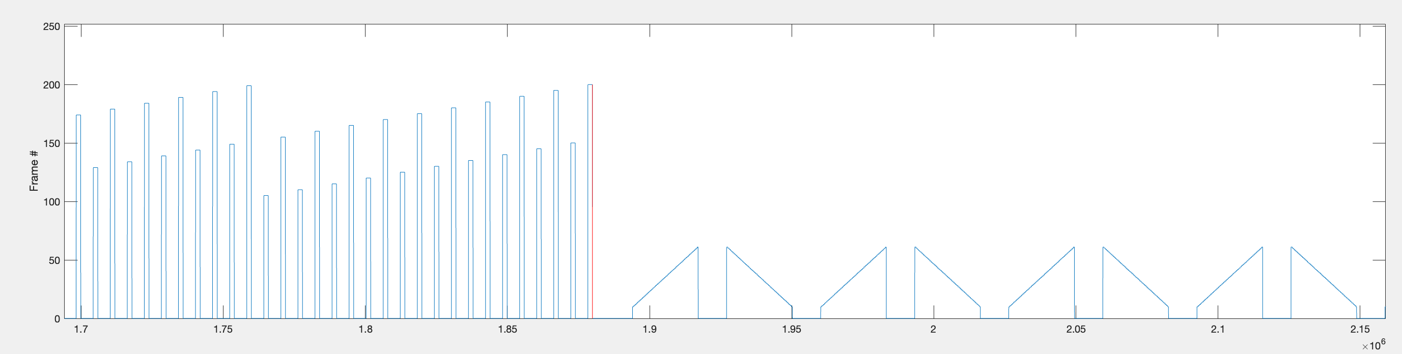
Similar to how the bar data is parsed, the difference between the frame positions is used to coarsely divide the data up into the different stimuli. For the flash stimuli the variable idx contains the timepoints that correspond to the start of the different flash stimuli repetitions (both the 4 pixel and the 6 pixel flashes).

As a reminder, P2 consists of 4 pixel flash stimuli presented, followed by 6 pixel flash stimuli of one contrast (designated by the value of the parameter on_off). Both the ‘on’ and the ‘off’ versions of P2 use the same pattern files that contain frames with dark flashes followed by frames with bright flashes. It is only the position functions, the files that tell the controller which frame of the pattern to present, that differ between the ‘on’ and ‘off’ versions of P2. Because of this, a key difference then between the ‘on’ and ‘off’ versions of P2 is that the first flash of both the 4 pixel and 6 pixel flashes for the ‘off’ version is frame 2 of the pattern - which is equal to the value 1 in f_data. Whereas in the ‘on’ version of P2, the first flash of the 4 pixel flashes is f_data = 197 and the first flash of the 6 pixel flashes is f_data = 101. This is because there are 196 4 pixel dark flashes and 100 6 pixel dark flashes in the pattern before the bright flashes. This information is used to find the start of the 4 pixel flashes and the 6 pixel flashes.

To find the end of the flash stimuli repetitions, the beginning of the 6 pixel flash stimuli is used to set the end of the 4 pixel flash stimuli. The end of the 6 pixel flash stimuli is found using the same method that is used when parsing the bar data. These timepoint indices are stored in idx_6px.

[ PNG - 0014 ] ^ f_data with vertical lines for the beginning of each flash stimulus - OFF STIMULUS.

[ PNG - 0015 ] ^ close up of 0014 for the start of 4px flashes - rep 1.

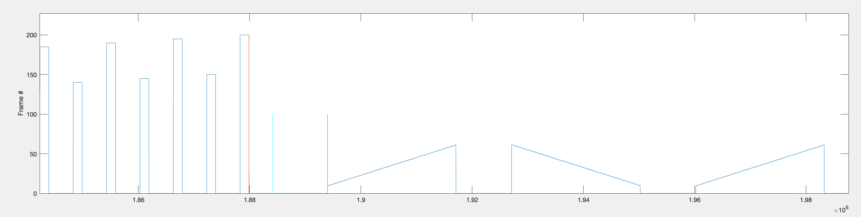
[ PNG - 0015-5 ] ^ f_data with vertical lines for the beginning of each flash stimulus - ON STIMULUS.

Find the timepoints for when individual flash stimuli start and stop.

start_flash_idxs is then generated that contains the timepoints within the range of the flash repetitions where the difference in frame position is >0 - this happens whenever a flash starts. These indices are then used to extract the frame data and voltage data per flash. For each flash, the data extracted includes 1000 datapoints before the flash starts until 6000 datapoints after the flash starts. As of July 2025, both the 4 and 6 pixel flashes are presented for 160ms then have a 440ms interval before the next flash starts. 160+440 = 600ms = ~6000 datapoints. So, the data extracted includes 1000 datapoints before the flash starts until just before the next flash starts. The timeseries of frame data is stored within the array data_frame of size [n_reps, 7000], the median-subtracted voltage data is stored in the array data_flash of size [n_reps, 7000] and the raw voltage data is stored in the array data_flash_raw of size [n_reps, 7000].

[ PNG - 0016 ] ^ Red line shows the start of the first flash Cyan line shows the actual range of timepoints for the first flash - 1000 timepoints before to 6000 timepoints after.

Compute metrics across flash reps and for the mean flash response.

A number of metrics are then calculated for each individual flash position including the variance across and within reps, the maximum and minimum voltage during the rep and the difference between the maximum and the minimum response. These metrics are then used to assign each flash position to a cmap group for later plotting. Basically, flash positions that showed a large depolarising response get assigned to group 1 and will have a warm colourmap in the heatmap plot, flash positions in group 2 have a large hyperpolarising response and will have a cool colourmap and flash positions that don’t have a big enough difference in their maximum and minimum voltage across the flash presentation are assigned to group 3 and will be white in the heatmap.

Plotting the flash data

Within process_flash_p2, the code loops through the 4 pixel size flashes and then the 6 pixel size flashes. It makes two receptive field plots for both and stores metrics about the voltage data and the receptive field size and shape in a nested structure rf_results.

Grid format plot with the mean timeseries of each flash response and the subplot’s background colour-coded by the cmap_id value and data_comb value. (src/analysis/plotting/plot_rf_estimate_timeseries_line)

This figure contains the mean voltage timeseries per flash position organised by its location in space (corresponding to its position on the screen from the fly’s perspective). The voltage data is downsampled by 10 to try and reduce the size of the figure slightly. If a flash position subplot is assigned cmap_id of 1 or 2 then it’s background is filled with a uniform red or blue background, respectively. The intensity of the background is proportional to that flash position’s data_comb value that is linked to it’s absolute maximum or minimum voltage. These values were normalised between 0 and 1 before passing the array into the function. So, flash positions with the highest maximum voltages will have the darkest red backgrounds and flash positions that elicited the lowest minimum voltage will have the darkest blue backgrounds. Flash positions with cmap_id value = 3 will have white / grey backgrounds. The resultant_angle from the processing of the bar stimuli is passed through to this function and an arrow is overlaid on top of the subplots, positioned within the centre of the figure and pointing in the direction of the resultant_angle.

[ PNG - 0017 ] ^ Timeseries heatmap plot

Heatmap plot (src/analysis/plotting/plot_heatmap_flash_responses)

This function creates a heatmap of the normalised values within data_comb (values between 0 and 1) using a redblue colourmap. The colourmap is centred around the median value to get a good colour range and so that the median value is white.

med_val = median(data_comb(:)); clim([med_val-0.5 med_val+0.5])

[ PNG - 0018 ] ^ Heatmap plot

Calculating metrics from the flash data

The function src/analysis/protocol2/gaussian_RF_estimate fits and plots a rotated 2D Gaussian fit around the excitatory and inhibitory lobes of the receptive field. It takes in the normalised and unnormalised versions of data_comb as it’s inputs and uses the built in MATLAB function lsqcurvefit to optimise the parameters for the gaussian fit. The function generates multiple plots showing the fitted data for both the excitatory and the inhibitory lobes and returns the metrics: optEx - R_squared optInh R_squaredi f1 - fitted inhib plot f2 - fitted excite plot

[ PNG - 0019 ] ^ fitted excitatory plot

[ PNG - 0020 ] ^ fitted inhibitory plot