Characterisation of collective fruit fly behaviour to moving patterns

End-to-end pipeline for a high-throughput behavioural screen

End-to-end pipeline for high-throughput fruit fly behaviour: MATLAB stimulus protocols, automated Python processing, and a Dash dashboard for results.

Highlights

• Designed and ran a behavioural screen across 19 GAL4 driver lines that silence individual visual cell types to investigate the role of these cell types in walking fruit flies’ responses to moving stimuli.
• Wrote the MATLAB protocols that generate the visual stimuli on the lab’s custom LED arenas and synchronise each pattern to the behavioural camera.
• Automated the data pipeline across 3 networked machines: watch, transfer, validate, track, analyse. Including a pipeline status page that keeps track of where each experiment folder is in the process.
• Created several interactive resources (Dash dashboard, HTML trajectory viewer) that experimenters could use to interact with the data.

Background

When an animal moves, the whole visual world slides across its eyes. That pattern of apparent motion is called optic flow, and it is one of the most ancient cues available for working out how you are moving: walking forwards streams the world past you on both sides, while being rotated sweeps it in one direction across the entire visual field.

A fly that detects rotational optic flow it did not cause itself will turn in the same direction, as though to cancel it out. This reflex is the optomotor response, and it is one of the most dependable behaviours in experimental neuroscience — a precisely controllable stimulus producing a precisely measurable action.

Figure 1: Optic flow, and the response it drives. Left: walking forwards produces translational flow, streaming outwards past the fly. Middle: being rotated produces rotational flow, sweeping across the whole visual field in one direction. Right: a fly that did not initiate that rotation turns with it to cancel it out — a corrective course manoeuvre. Arrows mark optic flow (dark red), voluntary movement (grey) and involuntary movement (blue); the insets show the corresponding flow field. Fly illustrations made with BioRender.

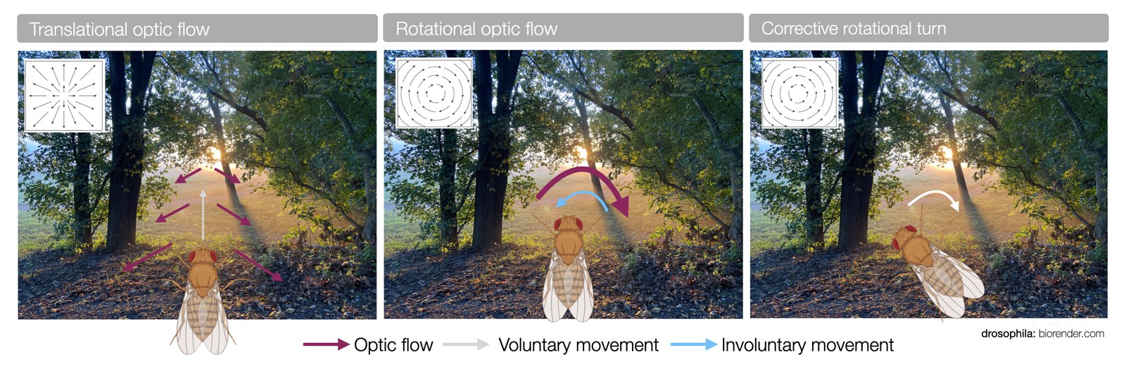
That dependability is what makes it useful. If you can switch off one cell type in the visual system and watch the response change, you have a way of asking which neurons the behaviour actually depends on and try and work out what visual information that specific cell type actually cares about. Most of what is known about the optomotor response, though, comes from flies that are tethered in place or walking or flying alone.

We measure it instead in groups of ~fifteen freely walking flies, in an arena large enough that they can walk as they like. The main reason is throughput - every trial reports on fifteen animals rather than one - but testing flies together also lets us ask whether any collective behaviour emerges when a group experiences the same moving pattern at once.

Problem

Build the system to perform a high-throughput screen. This includes: generating the visual stimuli, creating a system for syncronising the different acquisition components and developing a robust processing pipeline for the resulting data.

Methods

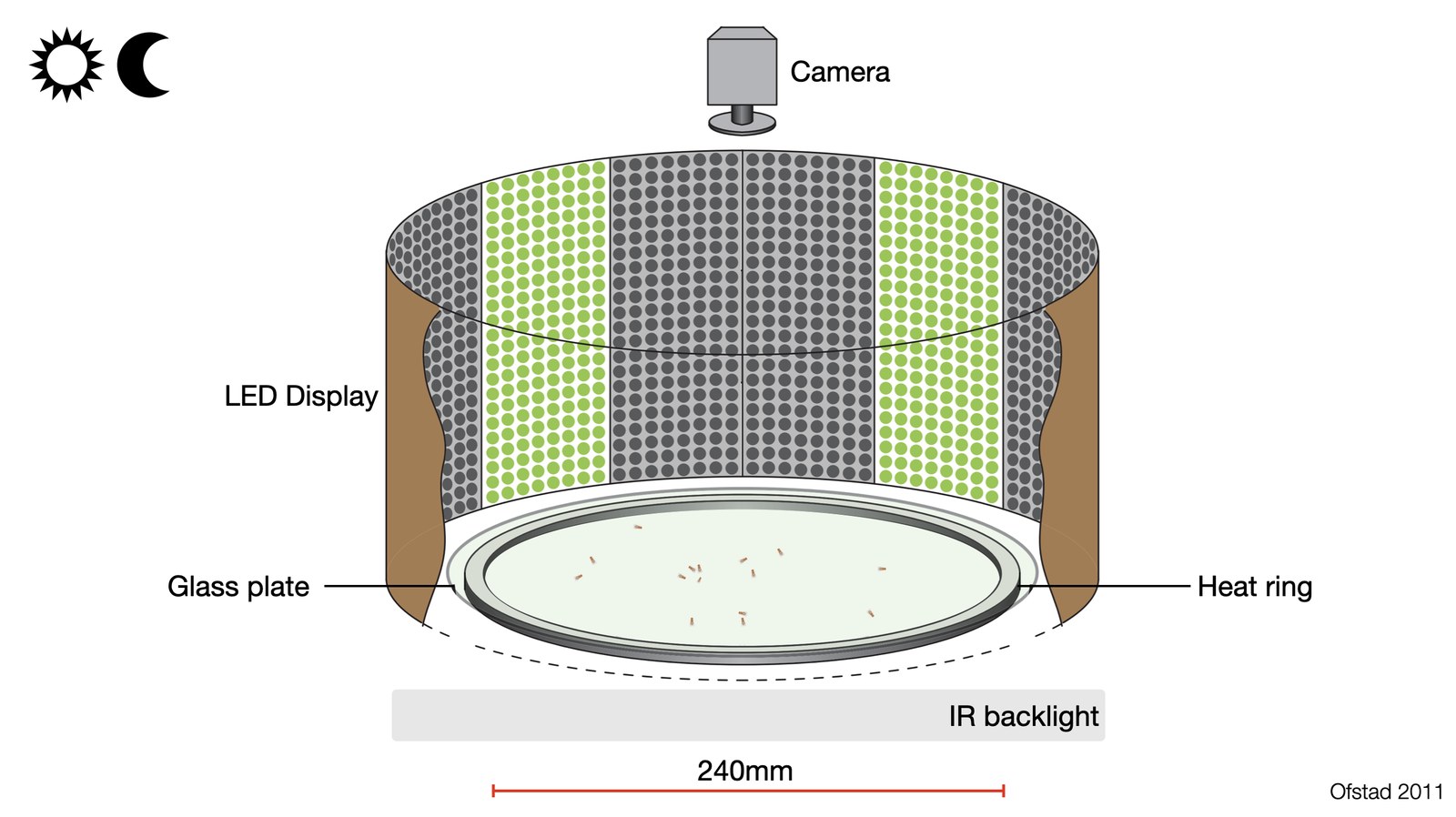
Experiments run in a circular arena 24 cm across, which is large by the standards of fruit fly neuroscience. LED panels line the walls facing inwards to present the moving patterns, an infrared backlight underneath silhouettes the flies for the camera above, and a heated ring around the perimeter keeps them away from the edge. The panels are a modular system designed and built in the lab, and are documented in their own right at Modular LED Displays.

Figure 2: The behavioural rig. LED panels line the arena wall facing inwards to present the moving patterns, an infrared backlight below silhouettes the flies for the camera above, a glass plate forms the floor, and a heated ring around the perimeter keeps the flies away from the edge. The scale bar gives the arena diameter: 240 mm. Adapted from Ofstad et al. 2011.

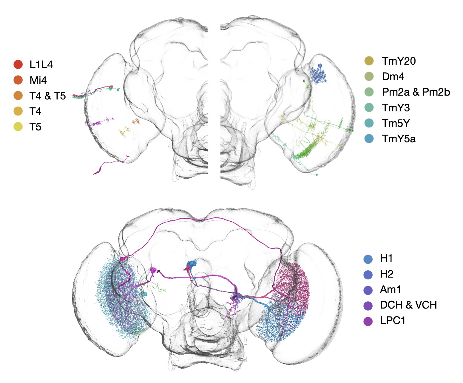
The screen takes advantage of the fruit fly’s genetics. A GAL4 driver line restricts expression to a chosen population of cells, and pairing it with a shibire-kir effector silences those cells specifically. Each line in the screen therefore asks the same behavioural question of a different component of the motion vision circuit, and the cell types chosen are those already thought to carry motion information through the visual system.

Figure 3: Example neurons from the cell types targeted in the screen, all thought to carry motion information through the visual system. Top: columnar and small-field types, including the direction-selective T4 and T5 neurons. Bottom: wider-reaching neurons — H1, H2, Am1, DCH/VCH and LPC1 — several of which cross between the two optic lobes. Colours correspond to the labelled legends. Rendered from the male optic lobe connectome with code published in Nern et al. 2025.

Before any of those lines were run, I spent a series of test protocols on the control line establishing which stimulus parameters drew out the strongest, most consistent responses. Those tests produced one standard protocol, which was then frozen and used unchanged on every line in the screen — so differences between lines reflect the flies rather than the stimulus.

Because the flies are tested in groups, we also run control experiments on individual flies. If a group result holds up in a fly walking on its own, we can be confident it is a response to the moving pattern rather than flies simply steering around one another.

Figure 4: A trial as the camera sees it, looking down on the arena floor. Each coloured trace is the path of one fly, with around fifteen in a trial; the green and black bars ringing the arena are the moving grating they were shown, superimposed onto the video frame.

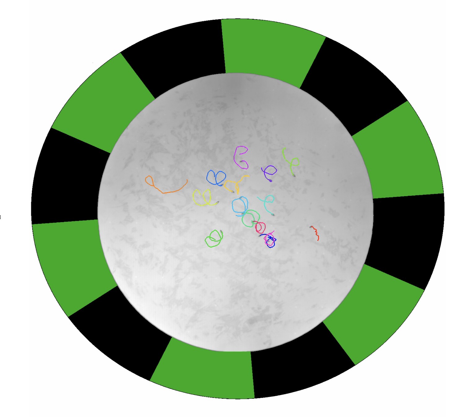
I built the pipeline that carries an experiment from the arena to a result. The stimulus code generates the patterns and the protocols, logs what was shown and keeps it synchronised with the behavioural camera. Everything downstream is automated across three machines: a service watches for new experiment folders, moves them to the institute’s server, and pulls a local copy onto the analysis computer — which matters mainly because it means the acquisition computer is never tied up processing, and experiments can keep running while the previous day’s data is worked through. Each folder is then checked to confirm the data looks as it should before tracking — with FlyTracker — and analysis run, with parameters held in one central configuration rather than scattered across the three machines.

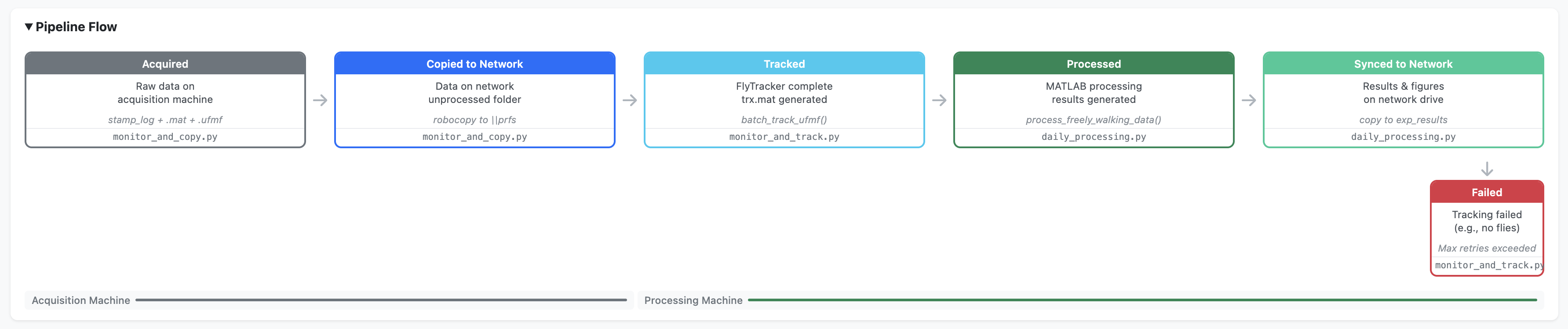
Figure 5: The stages an experiment passes through, from raw data on the acquisition machine to results and figures synced back to the network drive. Each box names what exists at that stage and the script that gets it there; the bars underneath show which machine does the work. Tracking is done with FlyTracker, and a run that fails — no flies detected, say — is tagged Failed once it exceeds its retry limit. These are the tags the pipeline status page reports.

The stage labels in that flow chart do real work. I built a pipeline status page that looks across both computers and the server at once, lists every experiment folder and tags it with how far through the pipeline it has reached. It earned its keep while the screen was running: a folder that stalled mid-transfer, an experiment that failed part-way through, or a dataset that processed incorrectly all surface immediately, rather than being discovered weeks later.

Two more tools came out of the analysis side. The first is an interactive Dash and Plotly dashboard covering the whole dataset, with statistical comparisons built in for spotting outliers — it runs locally, since it needs the raw data files, and it is what I open when someone wants to see results there and then. Its documentation walks through the views and how to launch it. The second is a standalone HTML trajectory viewer, which reads compressed JSON files holding a subset of the data. That combination can be emailed to a collaborator who can then explore individual flies’ trajectories and metrics in their browser, with nothing to install and no access to the server required.

Figure 6: Two views of the dashboard. Left: every stimulus condition overlaid for a single strain — here mean angular velocity across the trial — with the per-condition distributions underneath. Right: the summary heatmap, which compares each silenced line against the control across the behavioural metrics, above one metric shown as a timecourse and as a distribution. The sidebar sets the strain, the metric, and the quality-control and averaging rules applied throughout.

Figure 7: The trajectory viewer, a standalone HTML page that reads compressed JSON files holding a subset of the data. Left: the selected fly’s path through the arena. Right: its behavioural metrics aligned to the stimulus — angular and forward velocity, distance from centre, viewing distance, head-travel angle and tortuosity — with the current frame marked and the stimulus periods shaded.

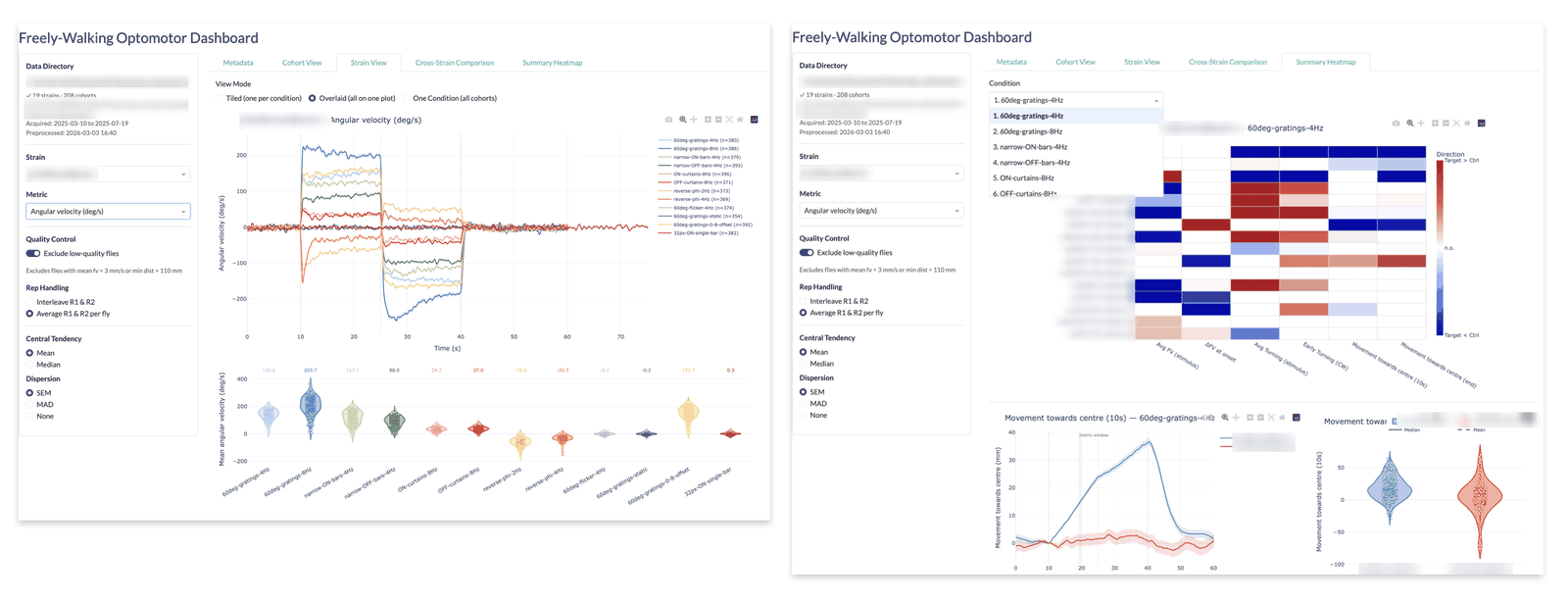
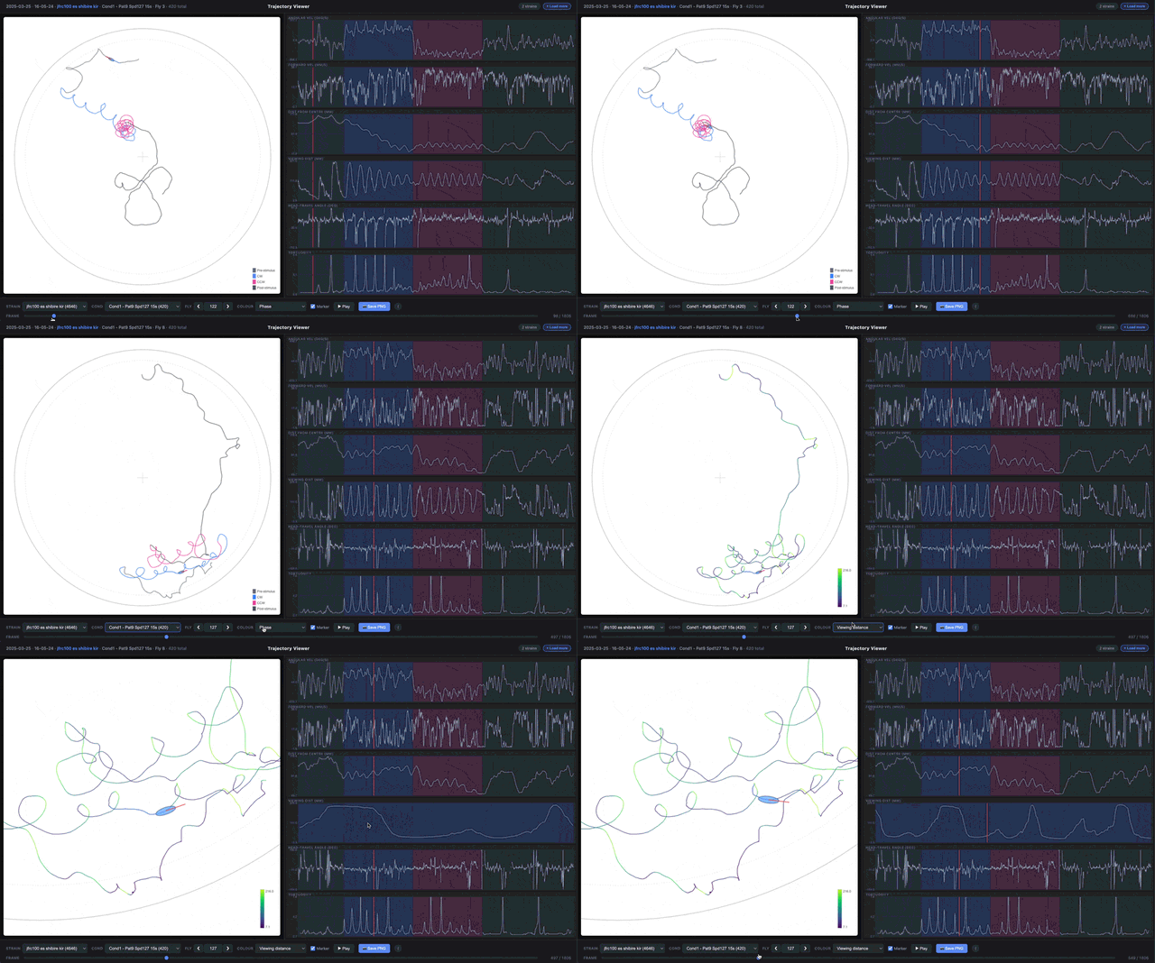
This was also the first project I documented properly. The documentation site covers the rig, the protocols, the pipeline and the analysis, and it exists because I wanted anyone joining the project to be able to run it without me sitting next to them — and because I suspect it will still be useful to someone here long after I have moved on. Part of that is an automatic experiment logging system: running a protocol pops up a short form, and MATLAB posts the answers straight into a Google Form, which collects every experiment’s date, protocol, strain, conditions and my notes on how the flies behaved into a single spreadsheet without anyone typing into one.

Outcome

The system was built and the first phase of the screen run on it: a frozen standard protocol, an automated path from arena to analysed result, a status page that surfaces failures the same day, and documentation so the project outlives my involvement.

We are in the process of writing up the results from this screen into an article for publication.

Links

• Source Code
• Documentation for this project — the rig, protocols, pipeline and analysis.
• Experiment logging system — how the Google Forms logging works, if you want to set up the same thing.
• Results dashboard — documentation for the Dash dashboard, including annotated screenshots of each view. The dashboard itself runs locally against the raw data.
• Modular LED Displays — documentation for the LED panel system the arena is built from.

References

• Ofstad TA, Zuker CS, Reiser MB. Visual place learning in Drosophila melanogaster. Nature 474, 204–207 (2011) — the source of the arena schematic in Figure 2.
• Nern, A., Loesche, F., Takemura, S., Burnett, L.E., et al. Connectome-driven neural inventory of a complete visual system. Nature 641, 1225–1237 (2025) — the connectome the cell type renders in Figure 3 come from.

Acknowledgements

This project took place while I was a member of the Reiser Lab at Howard Hughes Medical Institute (HHMI) Janelia Research Campus. The project came about while I was supervising our summer intern, Hannah-Marie Santos in the summer of 2024. In 2025, I worked closely with and mentored Aparna Dev, a member of Janelia’s Project Team Resources (PTR) and Grace Biondi, a graduate student in the Reiser Lab, and fly husbandry was carried out by Dr Ed Rogers throughout. Janelia’s Invertebrate Shared Resource helped maintain some of the fly stocks.