Pipeline for investigating neural responses to moving stimuli.

Highlights

Designed a two-stage adaptive protocol for patch electrophysiology.
Wrote the MATLAB stimulus generation and automatic logging code.
Built the analysis scripts that extract the receptive-field structure and quantify direction-selectivity indices for each cell, plus a Dash dashboard for reviewing recordings cell by cell.

Background

Direction selectivity has to be built somewhere. In the fly’s visual system, the first cells that respond more strongly to motion one way than the other are T4 and T5 — T4 to moving bright edges, T5 to dark ones. It is widely thought that everything downstream that cares about motion inherits its directional preference from them.

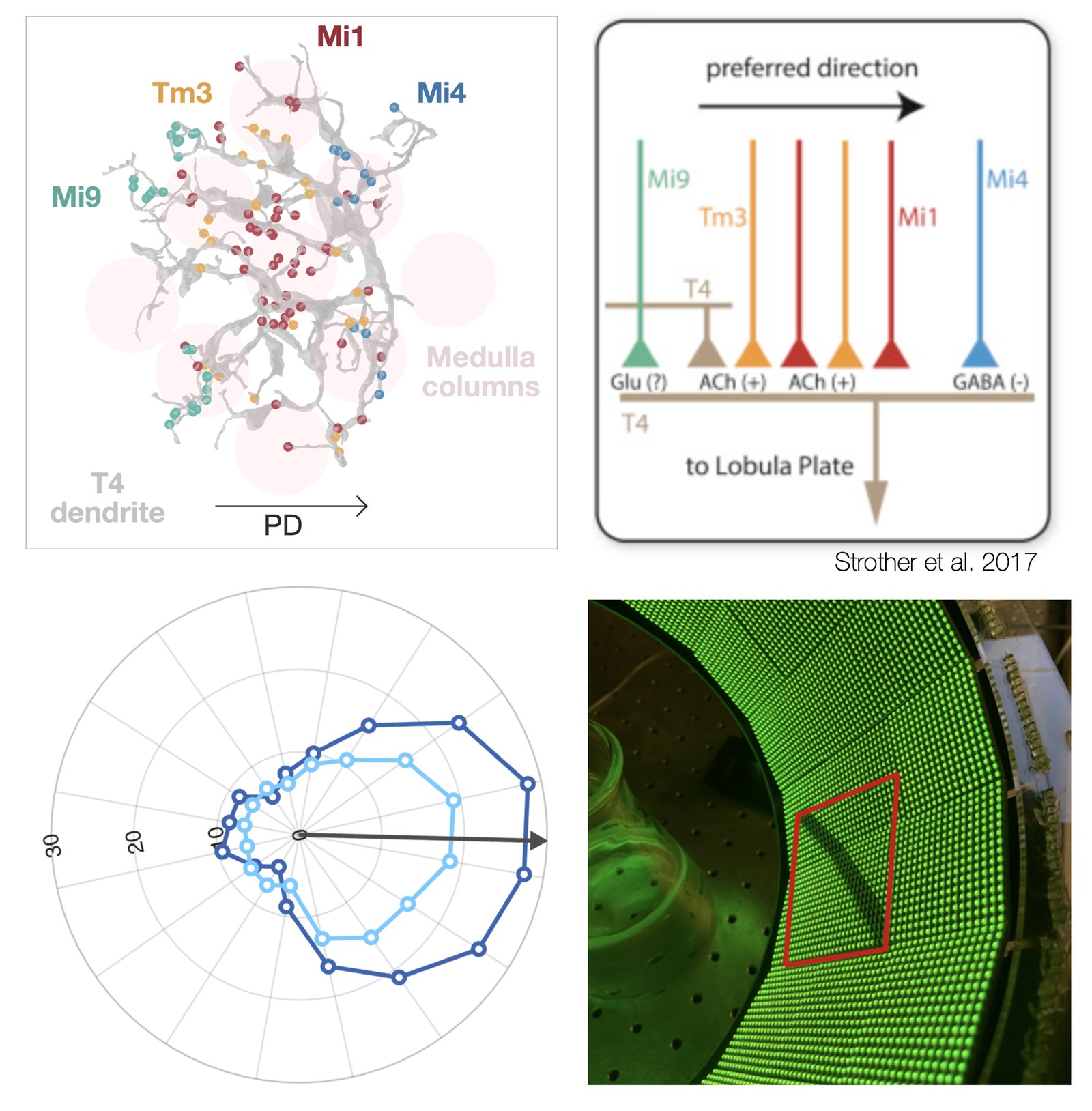
That preference comes from asymmetric inputs. A T4 or T5 cell collects excitation and inhibition from columnar neurons that synapse at different positions along its dendrite, and because the dendrite is laid out retinotopically, those positions correspond to different points in visual space. Mapping the receptive field with local flashes shows the consequence directly: offset depolarising and hyperpolarising fields, with fast excitation and an inhibition that is delayed and trails it in space. That was worked out for T4 in Gruntman et al. 2018 and for T5 in Gruntman et al. 2019 (both below). An edge sweeping one way arrives at the inhibitory field first and the response is suppressed; sweeping the other way it does not. The direction preference is a consequence of where the inputs sit, not only of what they are.

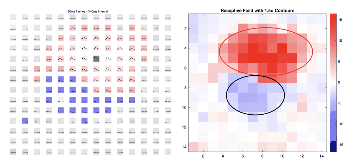
So the shape of a cell’s receptive field is the mechanism, not merely a description of it. Map it finely enough and the offset is directly visible: in the map above, a depolarising lobe sits above a hyperpolarising one, displaced in space. Perturb the wiring and you would expect that offset and the direction selectivity it produces to shift together — so it is worth measuring both in the same cell.

Figure 1: Where direction selectivity comes from, and how it is measured. **Top left:** the dendritic field of a single T4 cell (grey), with coloured circles marking synaptic inputs from different cell types — **Mi1**, **Tm3**, **Mi4** and **Mi9**. Pale pink discs are medulla columns; the arrow marks the cell’s preferred direction. **Top right:** the same inputs drawn schematically, in the same colours, arranged along the preferred-direction axis with their neurotransmitters and signs, feeding T4’s output to the lobula plate. Adapted from Strother *et al.* 2017. **Bottom left:** a single T4 cell’s response to bars sweeping in 16 directions, plotted as a polar tuning curve — dark blue at 28°/s, light blue at the faster 56°/s. **Bottom right:** the LED arena, with the region in which the sweeping bars are presented outlined in red.

The difficulty is time. An in vivo patch recording lasts only as long as the cell stays healthy, and mapping a receptive field at fine resolution across the whole arena is far too slow to fit inside that window — most of the positions tested would fall in parts of visual space the cell ignores. Fine mapping has to be aimed.

Problem

Recover both the fine structure of a cell’s receptive field and its direction selectivity from a single patch recording — by locating the receptive field quickly, then spending what time remains only where the cell actually responds.

Methods

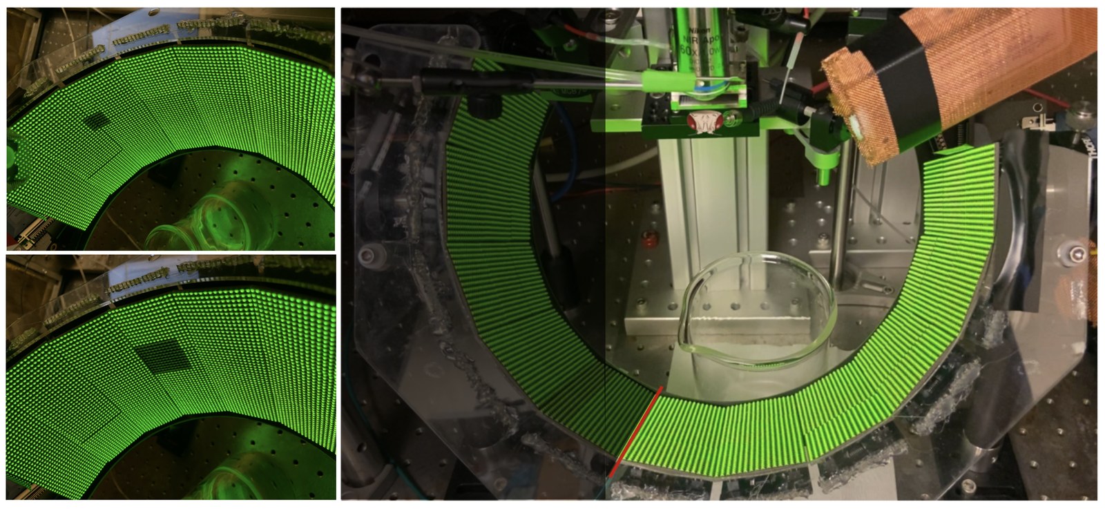
Both protocols run on the lab’s G4 LED arena, driven through its G4_Display_Tools experiment conductor.

Figure 2: The LED arena used for these *in vivo* patch clamp recordings. **Top left:** a 6 × 6 pixel flash on the display. **Bottom left:** a 12 × 12 pixel flash, for scale. **Right:** the whole rig from above, with the recording apparatus over the arena. The cartoon fly marks where the animal sits, and the shading covers the half of the arena that is never used — stimuli are only presented on one side.

The first protocol is a coarse survey, around seven minutes long. Bright and dark squares are flashed one position at a time across a grid spanning the arena, first at 12 px and then at 6 px, which is enough to establish roughly where the cell’s receptive field sits and whether bright or dark flashes drive it. Processing scripts then turn those recordings into a grid of response traces, one tile per position — the left-hand panel of the figure above is one of these.

At that point the experimenter reads the peak position off the grid and types it, with the arena side, into a short MATLAB GUI. That hand-off is deliberate: judging which position genuinely drove the cell is a call worth a human making, and it costs one number. Everything downstream of it is automatic. generate_protocol2() writes a complete second experiment into a timestamped folder — patterns, display functions, the experiment file and its log — generated from scratch and centred on the position just entered.

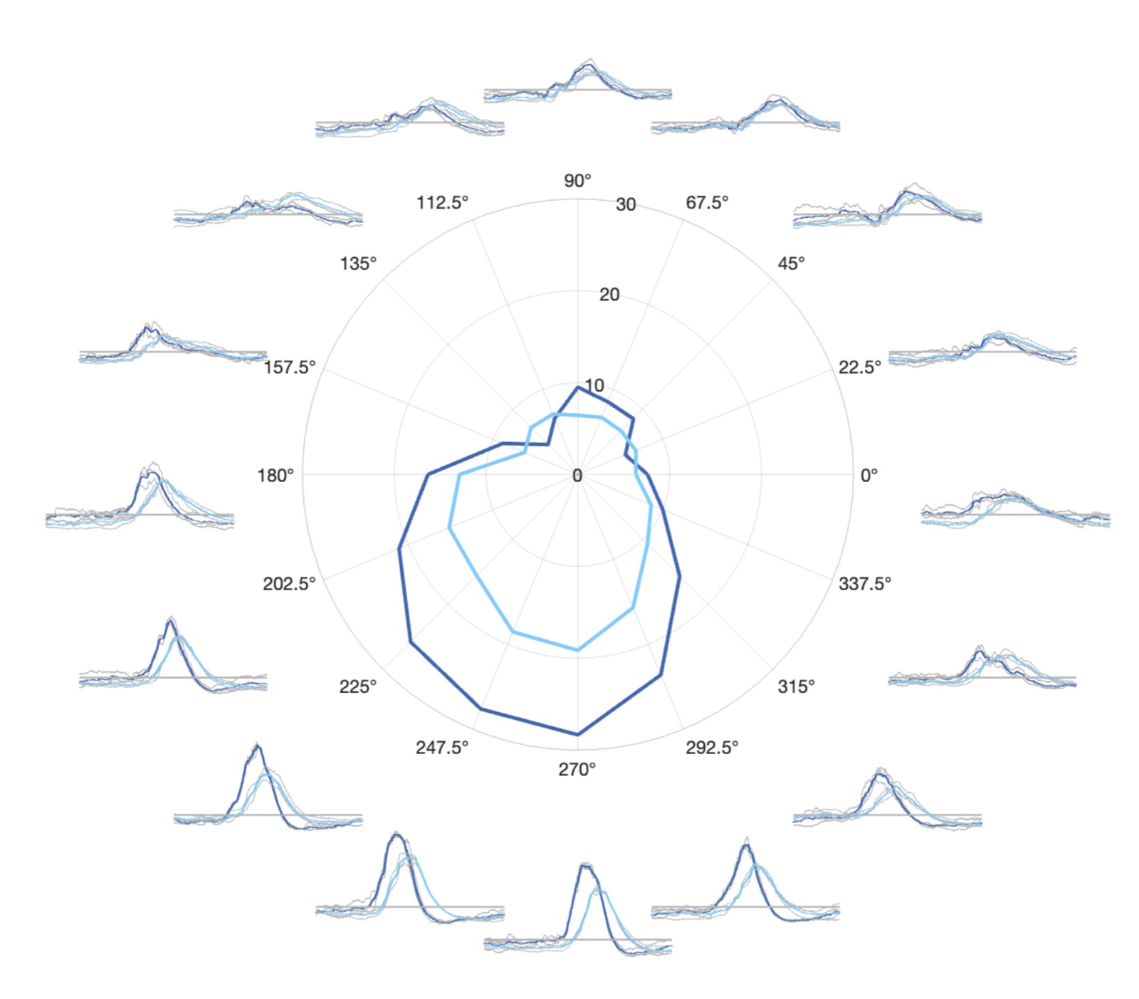
The second protocol runs for twenty to twenty-five minutes and does two things at once. Small squares, 6 px then 4 px with 50% overlap between positions, map the receptive field at much higher spatial resolution than the survey could afford. Moving bars, at two widths and at 14, 28 and 56 °/s in both directions, measure direction selectivity over the same patch of visual space. Because both are aimed at the region the cell responds to, almost none of the recording is spent on stimuli it will ignore.

Analysis is automated from there: receptive-field structure and centroid from the flash responses, direction-selectivity indices and median membrane voltage from the bar sweeps, alongside recording-quality checks that flag cells worth excluding. Results are collected into a Dash dashboard where each cell can be reviewed on one page — bar sweeps, both flash maps, bar flashes and the original survey grids — and experiment metadata is pushed to a shared Google Sheet so the log keeps itself.

Figure 3: The same cell’s direction tuning as in Figure 1, with the underlying recordings shown. The polar plot in the centre repeats the tuning curve — dark blue at 28°/s, light blue at 56°/s — and each surrounding trace is the membrane-voltage response to bars sweeping in that direction, positioned at the angle it corresponds to. Thin grey lines are individual repeats.

Outcome

The protocol is in routine use for the collaboration it was built for, and has been run across control and experimental genotypes to compare receptive-field structure and direction selectivity between them.

Links

Source Code
Documentation — how to generate and run both protocols, and how to analyse the data.

References

Strother JA, Wu ST, Wong AM, Nern A, Rogers EM, Le JQ, Rubin GM, Reiser MB. The emergence of directional selectivity in the visual motion pathway of Drosophila. Neuron 94, 168–182.e10 (2017) — the source of the input schematic in Figure 1.
Gruntman E, Romani S, Reiser MB. Simple integration of fast excitation and offset, delayed inhibition computes directional selectivity in Drosophila. Nature Neuroscience 21, 250–257 (2018) — the ON pathway (T4).
Gruntman E, Romani S, Reiser MB. The computation of directional selectivity in the Drosophila OFF motion pathway. eLife 8:e50706 (2019) — the OFF pathway (T5), and the protocol this one was based on.

Acknowledgements

The protocol was based on one developed by Dr Eyal Gruntman in the Reiser Lab.

This project took place while I was a member of the Reiser Lab at Howard Hughes Medical Institute (HHMI) Janelia Research Campus. The in vivo patching experiments were carried out by Dr Jin-Yong Park, a member of Janelia’s Project Team Resources (PTR). Fly husbandry was carried out by Dr Ed Rogers, and Janelia’s Invertebrate Shared Resource helped maintain some of the fly stocks. The experiments were run for a collaboration with Dr Piero Sanfilippo in Dr Larry Zipursky’s group at UCLA.